Complete Camera Calibration Guide: Monocular, Binocular, Hand-Eye, and Surround View (2026)

Key Takeaways

• Camera calibration solves three core problems: intrinsic parameters (focal length, principal point), extrinsic parameters (camera position/orientation), and lens distortion correction
• Not all cameras need calibration — only cameras that participate in algorithmic computation (object detection, distance measurement, 3D reconstruction) must be calibrated
• Four coordinate transforms: World → Camera (rigid body via R,t) → Image (perspective projection) → Pixel (discretization). This is the complete pipeline
• Reprojection error < 0.3px is not enough — calibration must be validated with independent test sets, straight-line verification, physical object ranging, and sensor fusion alignment
• Binocular adds two steps: stereo calibration (baseline R,t) and stereo rectification (epipolar error < 0.25px). Hardware trigger sync is mandatory
• Multi-camera joint calibration unifies all cameras into one coordinate system. Four methods: common target, chain calibration, motion-based, natural scene
• Temperature drift is real: every 10°C change shifts focal length by 0.3-0.5%. Online self-calibration is the long-term solution
• Aomway applies these same calibration principles in its multi-antenna and video transmission systems to ensure consistent RF performance across production units

Camera calibration covers four main threads — monocular handles intrinsic parameters and distortion, binocular handles stereo ranging, hand-eye calibration handles robotic arm coordination, and surround view handles vehicle panoramic stitching. This guide breaks down each thread with flowcharts and troubleshooting sequences.

---

1. What Problem Does Camera Calibration Solve?

Cameras capture 2D pixel arrays; the real world is 3D. For robots or autonomous driving systems to understand the real world through images — such as measuring obstacle distance or determining lane line positions — a mapping between pixel coordinates and real-world coordinates must be established.

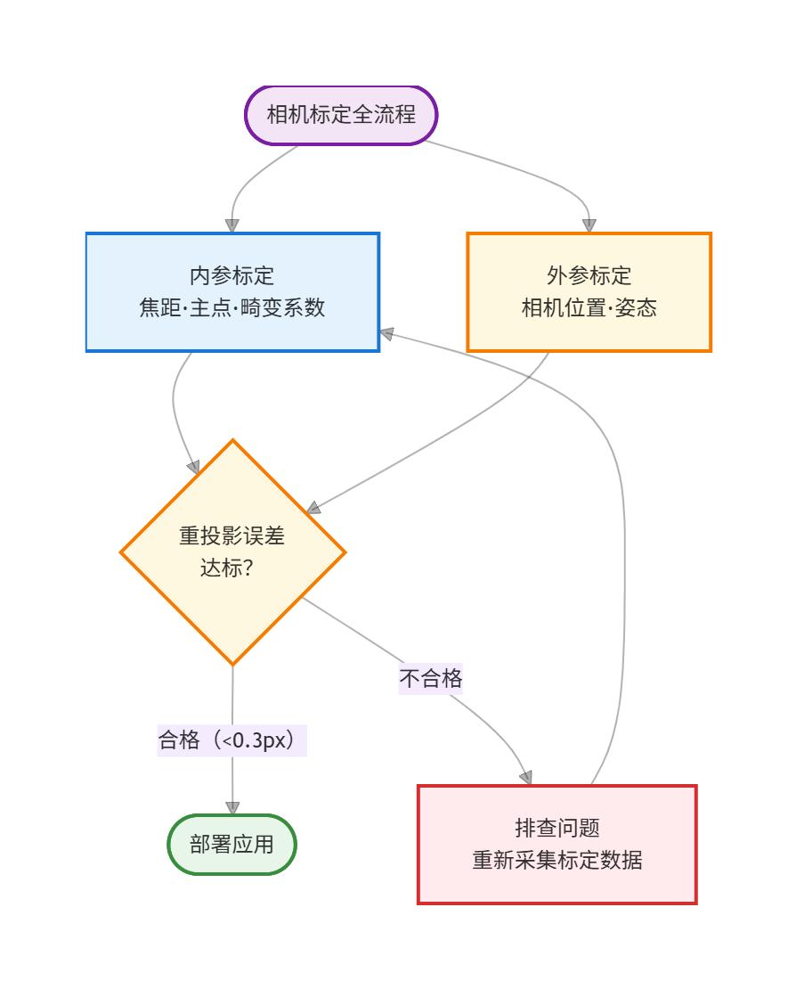
This mapping is what calibration does. Broken down into three core problems:

1. Intrinsics: What angle in the real world does each pixel correspond to? Where is the image center? How much does the lens bend the image?
2. Extrinsics: Where is the camera mounted on the vehicle/robot? Which direction does it face? How does it relate to the vehicle/robot body frame?
3. Distortion: Lenses bend straight lines — wide-angle lenses especially. How is this corrected?

Key judgment: Not every camera needs calibration. If the camera is for human viewing (backup camera, surveillance), calibration is unnecessary. But if images participate in algorithmic computation — object detection, distance measurement, 3D reconstruction — calibration is mandatory.

The complete calibration workflow looks like this:

2. Calibration Principles: Four Coordinate Transforms

Camera calibration essentially solves the transform relationships between four coordinate systems:

2.1 Four Coordinate Systems Quick Reference

Coordinate System	Dimensions	Origin	Unit	Meaning
World	3D	User-defined (vehicle center / calibration board corner)	meters / mm	Physical world reference
Camera	3D	Camera optical center	mm	Objects as seen from the camera
Image	2D	Optical axis intersection with image plane (principal point)	mm	Position on the physical image plane
Pixel	2D	Top-left corner of image	pixels	Final digital image row/column

2.2 Three-Step Transformation

Step 1: World → Camera (Rigid Body Transform)

Using rotation matrix R (3×3) and translation vector t (3×1), transform world-coordinate points into camera-coordinate points. R and t together form the extrinsic parameters.

Step 2: Camera → Image (Perspective Projection)

Using the pinhole camera model, similar triangles project the 3D point onto a 2D plane. The key parameter is focal length f.

Step 3: Image → Pixel (Discretization)

Convert physical dimensions (mm) to pixel units. Each pixel has physical size dx × dy (mm/pixel). The principal point’s position in the pixel coordinate system is (cx, cy). Focal length f, principal point (cx, cy), and pixel size dx/dy together form the intrinsic matrix K.

One sentence summary: Extrinsics determine “where the camera is and where it’s pointing.” Intrinsics determine “how pixels map to the physical world.” Distortion determines “how much the lens bends.” All three are essential.

2.3 Where Does Distortion Come From?

The ideal pinhole model cannot describe real lenses. There are two types of distortion:

• Radial distortion: Light bends more at the lens edges, creating “barrel” or “pincushion” distortion. Described by k1, k2, k3.
• Tangential distortion: Lens and image plane are not perfectly parallel. Described by p1, p2.

Key point: More distortion parameters are not always better. For typical scenes, k1, k2, p1, p2 (5 parameters total) are sufficient. Too many parameters risk overfitting, producing worse correction than a simpler model.

---

3. Calibration Parameters: How Intrinsics and Extrinsics Are Obtained

3.1 Intrinsics: Can Factory Values Be Used Directly?

Most industrial and automotive cameras come with factory intrinsic reports containing focal length, principal point, and distortion coefficients. These are measured on precision optical benches, theoretically very accurate.

But the problem is: factory conditions differ from actual deployment. Temperature changes, vibration, and lens thread tightness all affect intrinsic parameters — especially focal length. A 1% focal length error can produce a 1-meter measurement error at 100 meters.

Self-calibration optimization: Before deployment, recalibrate with a calibration board for more accurate parameters:

1. Print a high-precision checkerboard (commonly 9×6 or 10×7, each square size precisely known, e.g., 30mm)
2. Capture 15-30 images from varying angles and distances
3. Use OpenCV’s cv2.calibrateCamera() or MATLAB’s Camera Calibrator toolbox
4. Use reprojection error as quality metric: typically < 0.3 pixels, excellent < 0.1 pixels

Field experience: Factory calibration values are a fine starting point, but once the camera is mounted on a vehicle or robot, strongly recommended to recalibrate. Focal length and distortion coefficients can deviate noticeably from factory values under real-world conditions.

3.2 Extrinsics: Must Be Recalibrated After Mounting

Once the camera is installed on a vehicle or robot, the extrinsics (R, t) completely change. Extrinsics describe the camera coordinate system relative to the vehicle body/robot base.

Two common approaches:

• Static calibration: Place known markers around the vehicle/robot (calibration board, AprilTag, Charuco board), capture images, and solve via PnP (Perspective-n-Point) algorithm
• Dynamic calibration: Use vehicle/robot motion (straight line, turning) combined with odometry or IMU data for online visual-inertial joint optimization

Key point: Intrinsics can be “calibrated once, used long-term” (unless temperature changes drastically or the camera suffers physical impact). But extrinsics must be calibrated after mounting and require continuous online correction for drift during prolonged operation.

---

4. Monocular Camera Calibration

4.1 Five-Step Calibration Process

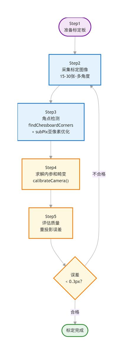
Step 1: Prepare the Calibration Board

Checkerboard is OpenCV’s natively supported pattern. Recommendations:

• Grid count: 9×6 or 10×7
• Grid size: 30mm or 50mm (select based on field of view)
• Print and mount on a rigid flat surface (glass or aluminum plate is best; paper on foam board lacks precision)

Step 2: Capture Calibration Images

• Capture 15-30 images with the board at various angles and positions across the field of view
• Cover the entire field: four corners, center, near, far
• Ensure the full board is visible in each image
• Tilt the board significantly (don’t keep it parallel to the image plane) — this better constrains focal length parameters
• Board should occupy 20%-60% of the image area

Step 3: Corner Detection

OpenCV provides cv2.findChessboardCorners() for automatic detection, paired with cv2.cornerSubPix() for sub-pixel refinement.

Step 4: Solve Intrinsics and Distortion

Call cv2.calibrateCamera() with world coordinates (known grid size) and image corner coordinates to output the intrinsic matrix K, distortion coefficients D, and per-image extrinsics R and t.

Step 5: Evaluate Quality

Calculate reprojection error: back-project the world corners using the calibrated parameters and compare with detected image corners. Average error < 0.3 pixels is acceptable, < 0.1 pixels is excellent. Above 0.5 pixels indicates corner detection issues or insufficient image quality — revisit the data.

Section summary: The five-step monocular calibration process — prepare board → capture 15-30 multi-angle images → detect corners → calibrateCamera() → evaluate reprojection error. Core principle: cover the entire field of view with varying board orientations, not just frontal shots.

4.2 Limitations of Monocular Calibration

A single camera cannot directly obtain depth information. After calibration, a monocular setup can only establish a “pixel → ray direction” mapping — it cannot determine distance along that ray. For ranging in robot/vehicle applications, monocular cameras must either pair with other sensors (IMU for scale estimation) or rely on ground plane assumptions.

4.3 How to Validate Calibration — Reprojection Error Alone Is Not Enough

Reprojection error < 0.3px is considered passing? Do not be fooled by this number. Reprojection error only tells you “the calibration board corners are well-fitted” — it does not guarantee the parameters work well in real-world scenarios. The following validation methods are ranked by reliability:

Method 1: Independent Test Set Reprojection Error

Use 20 images for calibration and set aside 5 images that never participate. Run cv2.projectPoints() on these 5 test images. If test set error is significantly higher than training error (e.g., 0.1px training vs 0.5px test), it indicates overfitting — insufficient pose coverage or too many distortion parameters.

Method 2: Straight-Line Verification After Distortion Correction

Photograph a scene with straight lines (corridor, building facade, tile floor). Apply distortion correction and visually check whether these lines are truly straight. This is the most intuitive validation — if corrected walls are still curved, the calibration has failed regardless of how low the reprojection error is.

Method 3: Physical Object Ranging (Binocular)

Place an object of known size at a known distance. Use calibrated parameters to compute depth. For example, place a calibration board at 1 meter — the measured distance should be 1.0m ± 2cm. A 10cm deviation means revisiting baseline distance and stereo rectification.

Method 4: Multi-View Projection Consistency (Multi-Camera)

Capture the same object from different positions. Use extrinsic parameters to project the object into a unified coordinate system and check projection point alignment. A deviation above 1 pixel indicates multi-camera extrinsic issues. Aomway uses similar multi-sensor alignment verification in its antenna array calibration process.

Method 5: Sensor Fusion Alignment Verification (Vehicle)

Project LiDAR point clouds onto the camera image and check whether point cloud edges align with image edges. For example, a street lamp pole’s point cloud should fall precisely on the pixel edge of the pole. A deviation of more than 5 pixels requires extrinsic recalibration. Tesla and other automakers use this as the core production-line acceptance criterion.

Real case study: After calibrating a binocular setup with a 0.12px reprojection error, the actual ranging error at 3 meters was 15cm. Review revealed all 20 calibration images were captured within the central 30% of the frame — the calibration board never appeared at the edges. The parameters fitted well in the center but extrapolated poorly at the edges. After adding 10 edge images and recalibrating, the ranging error dropped to 2cm.

Section summary: Low reprojection error ≠ good calibration. Must be validated with independent test sets, straight-line correction, physical object ranging, and sensor fusion alignment. The calibration board must cover frame edges, or extrapolation accuracy will be unreliable. Aomway applies these validation principles in its RF calibration workflows — no single metric is trusted in isolation.

---

5. Binocular (Stereo) Camera Calibration

5.1 What Does Binocular Add Over Monocular?

Binocular cameras not only need intrinsic calibration for each camera, but also the extrinsic parameters between the two cameras — the right camera’s position and orientation (R, t) relative to the left. This extrinsic is the foundation of stereo ranging: with the baseline distance and relative pose known, depth is calculated via triangulation from disparity.

5.2 Binocular Calibration Process

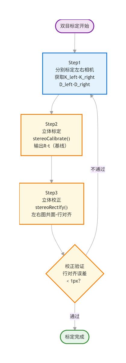
Step 1: Calibrate Each Camera Individually: Obtain intrinsic parameters and distortion coefficients for left and right cameras separately.

Step 2: Stereo Calibration: Use cv2.stereoCalibrate() with the same calibration board images captured by both cameras simultaneously. Output the rotation matrix R and translation vector t (baseline) between the cameras.

Step 3: Stereo Rectification: Use cv2.stereoRectify() to make the left and right images coplanar and row-aligned — the same object appears on the same row in both images. This is the prerequisite for stereo matching algorithms. Epipolar error should be < 0.25 pixels.

Step 4: Validation: Check the rectified image pair — the same feature point should lie on the same row (error < 1 pixel). Aomway stereo antenna tracking systems benefit from similar alignment validation procedures.

Section summary: Binocular calibration adds two steps over monocular — stereo calibration (find R,t baseline) and stereo rectification (row alignment). Epipolar error < 0.25px is a hard requirement. Hardware trigger sync is mandatory; software triggering is insufficiently precise.

5.3 Binocular Calibration Engineering Points

• Left and right cameras must be triggered simultaneously (hardware sync), or moving objects will produce disparity errors. Software trigger is typically insufficiently precise.
• Larger baseline improves long-distance ranging accuracy but increases near-field blind zone.
• Calibration lighting and temperature should approximate the actual operating environment.

---

6. Multi-Camera Joint Calibration

6.1 Why Joint Calibration?

Modern intelligent vehicles typically have 8-12 cameras (front, surround, side, rear), and robots may have multiple differently-oriented cameras. After individual calibration, all cameras must be unified into a single coordinate system — typically the vehicle body frame or robot base frame. This enables:

• 360° surround view stitching (Bird’s Eye View)
• Multi-camera object tracking (same object moving from one camera’s field into another’s)
• Multi-sensor fusion (camera + LiDAR + millimeter-wave radar)

6.2 Four Joint Calibration Methods

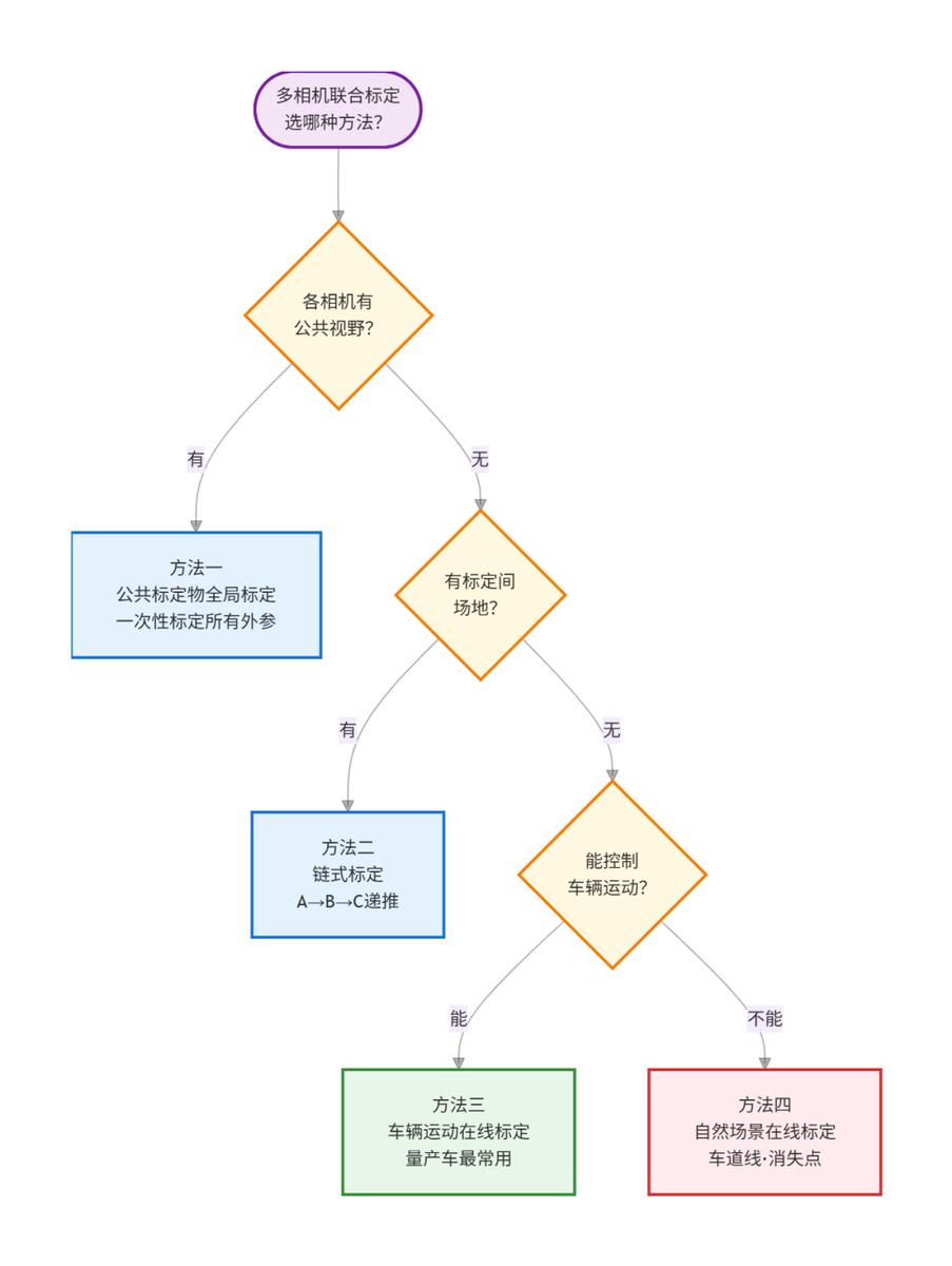
Method 1: Common Target Global Calibration: Place large calibration boards or multiple targets in an area visible to all cameras. Calibrate all extrinsic parameters simultaneously. High precision, but requires significant space, and multi-camera fields may not overlap.

Method 2: Chain Calibration with Overlapping Fields: Cameras A and B have overlapping views → calibrate A-B relationship. Cameras B and C have overlapping views → calibrate B-C. Derive A-C relationship, then unify to vehicle body frame. Suitable for surround-view systems.

Method 3: Motion-Based Online Calibration: Drive the vehicle along a fixed trajectory through a calibration zone. Using feature points (ground markers, wall markings) and vehicle odometry, simultaneously optimize all camera extrinsic parameters. This is the most common production-line approach.

Method 4: Natural Scene Online Calibration: Use lane lines, traffic signs, building edges, and other natural features for continuous online optimization. No dedicated calibration zone needed, but precision is lower than offline calibration. Suitable for long-term extrinsic maintenance and drift compensation.

Selection guide: Use Method 3 (calibration zone + vehicle motion) on production lines, Method 1 (common target) in R&D, Method 4 (natural scene) for long-term maintenance.

6.3 Key Challenges in Multi-Camera Calibration

Challenge	Description	Solution
No overlapping fields	Front and rear cameras see completely different areas	Chain calibration using vehicle motion constraints + odometry
Temporal sync	Multi-camera exposure timing drift > 0.1ms degrades accuracy	Hardware trigger + PTP time sync
Temperature drift	Long-term temperature changes shift mounting angles	Online calibration for continuous correction
Calibration venue	Sufficiently large calibration space required	Progressive calibration + natural scene assistance

Section summary: The core of multi-camera joint calibration is unifying the coordinate system. Choose the method by scenario. Temporal sync precision is a hard threshold — multi-camera systems must use hardware triggering.

---

7. Common Calibration Methods Comparison

7.1 Zhang Zhengyou Method (Most Mainstream)

Principle: Developed by Microsoft researcher Zhengyou Zhang in 1999. Uses a planar checkerboard captured from multiple angles. Solves intrinsics via homography matrix, then refines extrinsics through rotation matrix orthogonality constraints, with final LM nonlinear optimization.

Advantages:

• Only requires a planar calibration board — extremely low cost
• Easy to use — OpenCV/MATLAB/ROS all have ready implementations
• High precision — reprojection error can reach 0.1 pixels
• Robust — lighting variation has limited impact

Disadvantages:

• Requires 15-30 images at different angles
• Board must cover the entire field of view — large FOV needs large boards
• Less effective for wide-angle fisheye lenses (requires additional processing)

7.2 Tsai Two-Step Method

Principle: Solves most parameters linearly first, then uses nonlinear optimization for distortion coefficients. Two steps: coarse then fine.

Advantages: Lower computational cost than Zhang’s method — good for real-time applications.

Disadvantages: Slightly lower precision; requires higher-quality calibration targets (3D calibration object needed).

7.3 AprilTag / Charuco Calibration

Principle: Uses QR-code-like markers (AprilTag) or checkerboard+QR hybrids (Charuco). Each marker has a unique ID, so partial occlusion does not break calibration.

Advantages:

• Partial occlusion tolerated — great for multi-camera systems
• Full board visibility not required
• Higher corner detection precision

Disadvantages:

• Requires dedicated printed calibration boards
• Small markers difficult to detect at distance

7.4 Kalibr (Multi-Camera + IMU Joint Calibration)

Principle: Open-source calibration tool from ETH Zurich (GitHub: ethz-asl/kalibr). Supports multi-camera, camera-IMU, and camera-LiDAR joint calibration based on nonlinear optimization (Bundle Adjustment).

Advantages:

• Multi-sensor joint calibration supported
• Very high precision — used in academia and industry
• Supports AprilGrid calibration boards

Disadvantages:

• Steep learning curve
• Time-consuming calibration process
• High data quality requirements

7.5 Online Self-Calibration

Principle: Uses natural scene features (line features, vanishing points, lane lines) without any calibration board, dynamically updating extrinsic parameters during vehicle/robot operation.

Advantages:

• No calibration board or special venue needed
• Continuous extrinsic drift compensation
• Suitable for production-vehicle long-term maintenance

Disadvantages:

• Lower precision than offline calibration
• Depends on scene features — tunnels and night scenes may fail
• Complex algorithm requiring good initialization

7.6 Method Comparison Table

Method	Precision	Complexity	Cost	Best For
Zhang Zhengyou	High	Low	Very low	Monocular/binocular offline, R&D
Tsai Two-Step	Moderate-High	Medium	Low	Real-time applications
AprilTag/Charuco	High	Low	Low	Multi-camera, partial occlusion
Kalibr	Very high	High	Low	Multi-sensor joint, research
Online self-calibration	Medium	Low (use)	Needs dev	Production-vehicle extrinsic maintenance

Quick selection guide: R&D → Zhang’s method (lowest cost). Multi-sensor → Kalibr (highest precision). Production maintenance → Online self-calibration (continuous correction). Fisheye → Ocam model (mandatory for FOV > 150°). Aomway recommends matching the calibration approach to your accuracy requirements and production volume.

7.7 Fisheye Camera Calibration: Ocam Model

The above mainly covers standard lenses (FOV < 120°), but vehicle and robot applications frequently use fisheye lenses (FOV of 180° or more). The distortion is so severe that the traditional pinhole model plus radial/tangential distortion parameters is insufficient.

The Ocam model is the mainstream fisheye calibration approach. The core idea: use a polynomial to directly fit the mapping from incidence angle θ to image height ρ:

ρ = pol[0] + pol[1]·θ + pol[2]·θ² + ... + pol[N]·θ^N

where ρ is the pixel distance from the principal point, and θ is the angle between the incident ray and the optical axis. A 4-6 order polynomial is typically sufficient.

Ocam vs Traditional Distortion Model:

Feature	Traditional Model (k1,k2,k3)	Ocam Model
Applicable FOV	< 120°	180°+
Parameters	3-5	4-16 (adjustable)
Edge precision	Poor (unreliable extrapolation)	Good (global polynomial fit)
Math complexity	Low	Medium
OpenCV support	Native	Via cv2.fisheye or external libs

Engineering recommendations:

• Standard lens (FOV < 100°): Zhang’s method + 5 parameters (k1,k2,p1,p2,k3), OpenCV native
• Wide-angle (100° < FOV < 150°): cv2.fisheye.calibrate()
• Ultra-wide / fisheye (FOV > 150°): Ocam model via Kalibr or MATLAB

Relation to AVM systems: Typical AVM systems support both pinhole and Ocam models. In production, camera manufacturers use dedicated calibration equipment (precision turntable + collimator) for Ocam intrinsic calibration. The production line only performs extrinsic optimization. For R&D self-calibration of fisheye cameras, Kalibr’s AprilGrid + Ocam model approach is recommended.

---

8. Calibration Pitfalls and Common Mistakes

Calibration sounds straightforward — take some checkerboard photos, run an OpenCV function, get parameters. But in real engineering, calibration failures are extremely common. Here are six high-frequency pitfalls with real cases.

8.1 Insufficient Calibration Board Pose Coverage

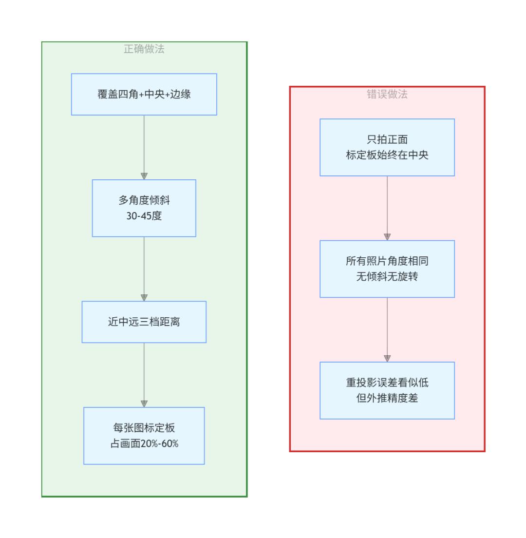
This is the most common problem. Many beginners take photos from a fixed position — only frontal shots, never tilting the board. The result: the board stays in the frame center, always parallel to the image plane.

Consequence: Focal length and principal point constraints are weak. The calibration looks good on reprojection error but produces terrible ranging accuracy.

Correct approach: The calibration board must cover the entire field — four corners, all edges. Tilt the board (at least 30-45 degrees), don’t keep it parallel. Capture near, medium, and far distances.

Real case: A lab calibrated a wide-angle vehicle camera with 20 images showing 0.08px reprojection error. On-road testing revealed 30cm lane detection deviation. All 20 images were taken from 1 meter directly in front — the board never appeared at frame edges. Adding 10 edge images and recalibrating reduced the deviation to 3cm.

8.2 Hand-Held Calibration Board

Many online tutorials demonstrate hand-held board capture, which causes multiple problems:

• Motion blur (even if the hand feels steady)
• Rolling shutter distortion (especially with consumer cameras)
• Temporal sync failure between binocular cameras (microsecond deviations cause significant errors)

Correct approach: Mount the camera on a tripod. Fix the calibration board on a stable surface. If you need to move the board, wait for stability after each movement before capturing. For industrial cameras, use hardware trigger sync.

Real case: A project used a USB binocular camera with hand-held calibration board. Reprojection error was 0.15px, but actual ranging at 2 meters showed 8cm error. Investigation revealed the USB camera used a rolling shutter — micro-shaking from hand-holding caused per-row exposure timing differences undetectable to the eye. Switching to tripod + hardware sync reduced the error to 1.5cm.

8.3 Improper Lighting

If the calibration board lacks sufficient contrast or has glare, corner detection fails silently.

Correct approach: Use uniform diffuse lighting (overcast outdoor, softbox). Avoid direct sunlight. Check images in real-time to ensure sharp black/white grid boundaries with no blown highlights or shadow loss.

Real case: An outdoor calibration at 3 PM with slanted sun caused half the calibration board to be overexposed. findChessboardCorners silently returned False for those images (no exception raised), so the calibration proceeded with only 8 effective frames instead of 20. Moving to shade restored 100% detection.

8.4 Too Many Distortion Parameters

OpenCV supports k1, k2, k3, p1, p2, s1, s2, s3, s4 — many parameters. Some practitioners enable everything, leading to overfitting: ridiculously low reprojection error but poor actual correction, especially at frame edges.

Correct approach: Simpler is better. Use k1, k2, p1, p2 for most scenes. Add k3 only if needed. Validate with independent test images, not just reprojection error.

Real case: An OpenCV forum user calibrated with an 8-parameter rational model, achieving 0.05px reprojection error. However, corrected images showed “waves” at the edges — straight lines were actually deformed after correction. The calibration data hadn’t covered frame edges, so the rational model made unreliable extrapolations. Switching to a 5-parameter model fixed the problem.

8.5 Ignoring Temperature Drift and Extrinsic Changes

Calibration is not a one-time process. Sensors operate from -20°C to +60°C, and temperature changes cause physical deformation and mounting angle shifts. Tesla FSD testing found that calibration deviations caused 23% of emergency braking failures.

Correct approach:

• Establish calibration parameter version management
• Periodically run full calibration verification on actual vehicles/robots
• Implement online calibration using natural features (lane intersections) for continuous optimization
• Calibration precision targets: camera ±0.1°, LiDAR ±0.2°, radar ±0.5°

Real case: A binocular camera calibrated outdoors in winter showed ranging accuracy drifting from 2cm to 8cm when used in summer. Temperature change from -5°C to 40°C shifted the focal length by approximately 0.4%, and the aluminum binocular bracket expanded. Adding an online calibration module that corrected extrinsics weekly using vanishing points stabilized ranging to within 2cm.

8.6 Calibration Board Quality Issues

Printing on plain A4 paper on an uneven foam board creates a “calibration board” with insufficient precision. Board flatness and grid size accuracy directly propagate into the calibration results.

Correct approach: Use high-precision rigid material boards (glass substrate, ceramic, aluminum). Grid size accuracy should be in microns. On a budget, at minimum use quality printing on glass or aluminum plate.

Real case: A team using A4 paper checkerboard on foam board found calibration results varied significantly between batches. Foam board warped by only 0.5mm under humidity changes, but this was enough to bias world coordinates. Switching to a $30 glass substrate improved reproducibility — batch-to-batch parameter variation dropped from 5% to under 0.5%.

8.7 Troubleshooting Flow — What to Do When Calibration Fails

When calibration results are unsatisfactory, follow this priority-ordered checklist to isolate the problem:

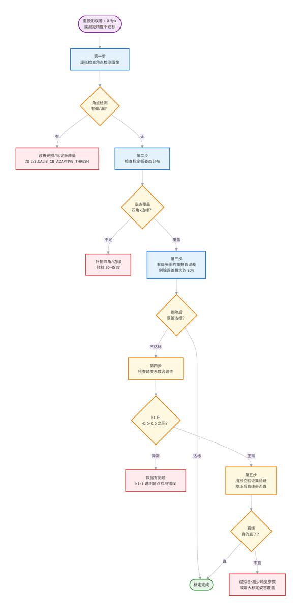
Mnemonic: First check corner accuracy, then pose coverage, then remove bad images, then check distortion reasonableness, finally verify with straight lines.

Step 1: Inspect each image’s corner detection. Draw detected corners (cv2.drawChessboardCorners()) and visually check alignment with black/white intersections. Off by more than half a pixel? That image’s data is contaminated. Common causes: uneven lighting, motion blur, board glare, low resolution. Fix: add cv2.CALIB_CB_ADAPTIVE_THRESH for low light, or remove the image.

Step 2: Check board pose distribution. Visualize each image’s extrinsic (rvec) to see board orientation distribution. If all poses cluster within ±10°, the board was never tilted — focal length constraints are weak. Ideally, the board should have distribution in X, Y, and Z rotational axes.

Step 3: Remove worst-error images. Each image has an individual reprojection error. Remove the worst 20% and recalibrate. If total error drops from 0.5px to 0.2px, those images had problems (poor corner detection or extreme pose).

Step 4: Check distortion coefficient reasonableness. Rule of thumb: k1 should be between -0.5 and 0.5. If |k1| exceeds 1 or especially 10, something is wrong — corner detection failure, grid size error, or all-frontal poses.

Step 5: Validate with independent test set. Don’t validate on your calibration data — that’s circular reasoning. Use a separate set for distortion correction and check whether straight lines are actually straight. If curves remain, reduce distortion parameters or improve pose coverage.

Section summary: When calibration fails, troubleshoot in order — corner detection → pose coverage → remove bad images → distortion coefficients → straight-line verification. Most problems are found in Step 1 or 2.

---

9. Calibration in Practice — Vehicle and Robot Applications

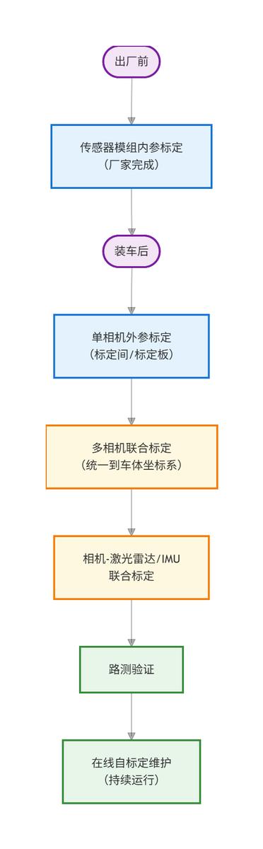
9.1 Vehicle Camera Calibration Typical Process

9.2 Robot Camera Calibration Typical Process

Robotic Arm Vision (Eye-in-Hand): Camera mounted on the robotic arm end-effector:

• Hand-eye calibration (Eye-to-Hand or Eye-in-Hand)
• Solve the transform from camera coordinate system to arm end-effector coordinate system

Mobile Robot Vision:

• Monocular/binocular/depth camera extrinsic calibration to robot base frame
• Visual-inertial joint calibration with IMU/odometry
• Online self-calibration to compensate for vibration and collision-induced extrinsic drift

9.3 Hand-Eye Calibration (Robot-Specific)

Robotics introduces a unique problem: the relationship between camera and robotic arm. Two configurations:

• Eye-to-Hand: Camera fixed in the workspace. Solve the transform from camera frame to robot base frame.
• Eye-in-Hand: Camera mounted on the arm end-effector. Solve the transform from camera frame to end-effector frame.

Mathematically: Solve the AX = XB equation. A is the arm’s end-effector motion (pose i → pose j), B is the observed calibration board motion, and X is the unknown transform from camera to arm end-effector (or base). Common algorithms: Tsai-Lenz (two-step, rotation then translation), Park method (Lie algebra based), Daniilidis method (dual quaternion for simultaneous rotation+translation).

Selection Guide:

Scenario	Approach	Typical Precision	Notes
Large-range (pick, sorting)	Eye-to-Hand	1-3mm	Recalibrate if camera moved
Fine operation (assembly, insertion)	Eye-in-Hand	0.5-1mm	Recalibrate on end-effector change
Both needed	Dual approach	—	Eye-to-Hand for coarse, Eye-in-Hand for fine

Common Hand-Eye Calibration Pitfalls:

1. Insufficient arm motion range: Swinging within 10° provides weak rotation constraints. Requires large motion in 3 orthogonal directions.
2. Degenerate board poses: Board always parallel to image plane makes PnP depth unstable. Multi-angle tilt required.
3. Arm kinematic error propagation: If the arm’s own kinematic accuracy is 2mm, hand-eye calibration will be no better than 2mm. Flexible joint arms need local-region calibration rather than full-space.

9.4 AVM Surround View System Calibration in Practice

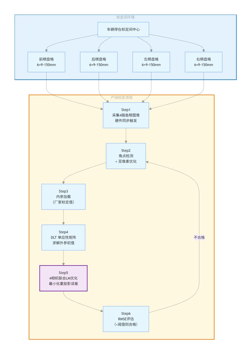
Automotive AVM (Around View Monitor) is the most typical camera calibration application in production vehicles. Here’s the breakdown for a 4-fisheye AVM system:

System Configuration:

• 4 fisheye cameras (front, rear, left, right), 1280×720 resolution
• Vehicle parked in calibration zone center, checkerboard patterns on the floor
• Each camera has a 6×9 checkerboard, each grid 100-150mm
• Calibration zone: approximately 6000mm × 6000mm

Core Algorithm:

1. Extrinsic Initial Value Calculation: For each camera, use detected checkerboard corners (world coordinates known) and corresponding image coordinates. Compute homography H via DLT + SVD decomposition. Decompose R and t from H: H = [r1, r2, t], where r1/r2 are the first two columns of the rotation matrix. Solve Euler angles (pitch/yaw/roll) via trigonometric functions.

2. Multi-Camera Joint LM Optimization: This is critical. Instead of optimizing each camera independently, all camera parameters (6 extrinsics per camera: 3 Euler angles + 3 translations) are placed in a single optimization problem minimizing total reprojection error across all cameras. This leverages the consistency of corner positions in overlapping regions as extra constraints, preventing each camera from “going its own way.”

3. Hierarchical Optimization: Three levels:

• Extrinsics only (6 params/camera) — production default
• Extrinsics + principal point (8 params/camera) — when lens mounting deviation is significant
• Extrinsics + principal point + FOV (10 params/camera) — when intrinsic fine-tuning is needed

4. Fisheye Model Support: AVM systems typically support both pinhole and Ocam models. The Ocam model uses a polynomial for the θ → ρ mapping without traditional distortion parameters — ideal for FOV > 180° fisheye.

5. Production Acceptance Criteria: Each camera’s reprojection error must be below a threshold (typically 1-2 pixels). All cameras must pass — a single failure triggers re-acquisition.

Differences Between Lab and AVM Production Calibration:

Dimension	Lab Calibration	AVM Production Calibration
Calibration board	Hand-held checkerboard	Fixed floor checkerboard (calibration zone)
Intrinsic source	Self-calibrated	Factory-provided + production fine-tuning
Calibration target	Full intrinsics + extrinsics	Extrinsics only (intrinsics pre-calibrated)
Optimization	Independent per camera	Multi-camera joint LM
Acceptance	Reprojection error < 0.3px	Reprojection error + stitching quality
Operator	Algorithm engineer	Production line worker
Cycle time	10-30 minutes	< 30 seconds

Why AVM Doesn’t Recalibrate Intrinsics on the Line: Fisheye intrinsics are highly nonlinear — calibrating them on a production line with limited checkerboard data is impractical. Camera manufacturers perform precision intrinsic calibration at the factory (turntable + collimator). The production line only optimizes extrinsics using the floor checkerboard. Unless the camera suffers severe impact or extreme temperature change, intrinsics remain stable.

AVM Consensus: Zhang’s method remains the foundation. 3D bowl projection works better than 2D planar projection (reduced edge distortion). GPU acceleration (OpenGL rendering) is key to achieving 30fps real-time stitching. Scene-feature-based online correction reduces LiDAR dependency. Aomway multi-antenna calibration processes use similar hierarchical optimization strategies to balance accuracy against production throughput.

Section summary: AVM production calibration and lab calibration are completely different — production requires completion within 30 seconds by line workers, using multi-camera joint optimization with factory-provided intrinsics. Hand-eye calibration’s core is solving the AX = XB equation, and arm kinematic error directly propagates into the calibration result.

---

10. Summary

Camera calibration is the foundation of robot and autonomous driving perception — directly affecting the accuracy of all downstream algorithms.

Category	Key Points	Key Metric
Intrinsics	Determines “how accurately the camera sees.” Factory values as initial guess, recalibrate after mounting	Reprojection error < 0.3px
Extrinsics	Determines “where and which direction.” Must be recalibrated after mounting; needs online correction long-term	Epipolar error < 0.25px (binocular)
Monocular	Simplest, cannot measure depth directly. Suitable for detection and classification	—
Binocular	Two extra steps (stereo calibration + rectification). Enables triangulation ranging	Hardware sync required
Multi-camera	Standard in production vehicles and complex robots. Core task: unify coordinate systems	Time sync < 0.1ms
Method	Zhang’s method is most cost-effective. Kalibr is most precise. Online calibration for maintenance	—
Validation	Reprojection error alone is not enough. Use independent test set + straight-line check + physical ranging	—
Troubleshooting	Check corners → check poses → remove bad images → check distortion → verify with lines	k1 range: -0.5~0.5
Temperature	Every 10°C shifts focal length 0.3-0.5%. Online calibration is the long-term safeguard	—
Hand-eye	Core equation: AX = XB. Arm kinematic error directly propagates	≥ 3 orthogonal motion axes
AVM	30-second production cycle, line worker operation, multi-camera joint optimization, factory intrinsics	—

Calibration is both simple and complex. Get the parameters right, and everything downstream works smoothly. Aomway applies these same calibration principles in its video transmission and antenna product testing, ensuring consistent performance across production volume.

Have questions about this article? Feel free to contact us at [email protected] — we’re happy to help!

Frequently Asked Questions

Q: When does a camera absolutely need calibration?

A: Any camera whose images participate in algorithmic computation — object detection, distance measurement, 3D reconstruction, SLAM, or sensor fusion — must be calibrated. Cameras for direct human viewing (reverse camera, surveillance monitor, video call) do not need calibration.

Q: What’s the minimum number of calibration images I need?

A: 15-30 images covering the full field of view with varying board orientations. Fewer than 10 images almost always produces unreliable results. More than 30 images offers diminishing returns unless you need very wide temperature or lighting coverage.

Q: Can I use factory calibration values directly?

A: As a starting point, yes. But factory values are measured on an optical bench under ideal conditions. After mounting on a vehicle or robot, temperature, vibration, and mechanical stress will shift the parameters. For best results, recalibrate after mounting and use factory values as an initial constraint.

Q: How do I know if my calibration is good enough?

A: Do not rely on reprojection error alone. Validate with: (1) an independent test set of images not used in calibration, (2) visual straight-line check after distortion correction, (3) physical distance measurement with a known-size object, and (4) cross-sensor projection alignment if available. Aomway uses multi-metric validation in all its RF and antenna production testing.

Q: How often should I recalibrate?

A: Intrinsics: recalibrate after any physical impact, extreme temperature exposure, or at least annually. Extrinsics: check and recalibrate after any mounting change. For production vehicles, implement online self-calibration using natural scene features for continuous drift compensation — especially important with seasonal temperature changes that can shift focal length by 0.3-0.5% per 10°C.