

Introduction: Why Noise Figure Is the “First Threshold” of RF System Design
At Aomway, our RF engineering team applies these noise figure principles daily in the design of high-performance drone video transmission systems and telemetry links. Understanding NF is not just academic – it directly determines flight range, video quality, and link reliability in real-world operations.
In modern wireless communications, radar, electronic warfare, and radio astronomy, receiver sensitivityis one of the most critical metrics for measuring system performance。Whether a receiver can reliably extract useful information under extremely low signal power conditions depends largely on its RF front-end Noise Figure (NF)。
The concept of noise figure may seem simple – it describes the degree of SNR degradation of a device or system as a signal passes through. In practical link budget engineering, precise NF calculation and optimization involves cascaded gain distribution、impedance matching、temperature compensation、frequency planning, and a series of other engineering details。every reduction of0.5 dB of system NF,can mean tens of kilometers of additional range、several percentage points of improved radar detection probability,or a satellite link margin going from”marginal”变为”robust”。
This article starts from the physical origin of noise, systematically explains the definition of NF, cascade calculation, quantitative relationship with receiver sensitivity, and provides practical design references for RF system engineers – methods that Aomway engineers apply daily in drone uplink and downlink design.
1. Thermal Noise: The Physical Foundation of All Noise Analysis
1.1 The Nature of Johnson-Nyquist Noise
Any resistive element above absolute zero temperature generates thermal noise。This phenomenon was first experimentally observed by J.B. Johnson in 1928, with the rigorous theoretical derivation provided by H. Nyquist shortly after.
The available noise poweris described by the classic formula – a formula that Aomway RF engineers reference daily in sensitivity budget calculations for long-range telemetry links.
N = kTB
其中:
- k is the Boltzmann constant, approximately 1.381 × 10⁻²³ J/K
- T is the absolute temperature (Kelvin, K)
- B is the system bandwidth (Hz)
This formula reveals an extremely important fact: thermal noise power is frequency-independent(within the microwave frequency range),It depends only on temperature and bandwidth. This uniform spectral distribution is why thermal noise is often called **”white noise”**。
1.2 Noise Power Density Under Standard Reference Conditions
In engineering practice, T0 = 290 K(约17°C)K is used as the standard reference temperature. Under this condition:
kT0 ≈ 4.00 × 10⁻²¹ W/Hz = -174 dBm/Hz
This -174 dBm/Hz is one of the most fundamental numbers in RF engineering. It means that at room temperature, any matched resistor produces approximately -174 dBm。
In a system with actual bandwidth B Hz, the **noise floor** is:
N0 = -174 + 10·log10(B) (单位:dBm)
For example, for a 1 MHz bandwidth system – typical for Aomway digital video transmission – the noise floor is:
N0 = -174 + 10·log10(106) = -174 + 60 = -114 dBm
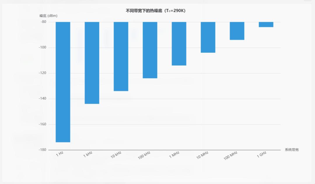
This chart clearly illustratesthe decisive impact of bandwidth on noise floor – every 10x increase in bandwidth raises the noise floor by 10 dB.This is the fundamental physical reason why narrowband systems inherently achieve higher sensitivity。
2. Noise Figure and Noise Temperature: Two Equivalent Languages
2.1 Rigorous Definition of Noise Figure
**Noise Figure (NF)**definition,originates from Harold Friis 在1944classic paper。Its essential meaning is:
The noise figure of a two-port network equals the ratio of its input SNR to output SNR – provided the input noise source temperature is the standard reference temperature T0 = 290 K。
Mathematically:
F = (SNRin) / (SNRout)
Where F is the linear noise factor. Converted to logarithmic form:
NF = 10·log10(F) (单位:dB)
一个An ideal noiseless devicehas a noise figure of 0 dB(F = 1),means the signal passes through without SNR degradation. Any real device–whether an amplifier、mixer, or filter–will introduce additional noise into the signal path,使得 NF > 0 dB。
2.2 Noise Characteristics of Active vs. Passive Devices
For passive devices(such as filters、attenuators、and transmission lines),its NF in numerical valueequals its insertion loss。For example, a bandpass filter with 3 dB insertion loss has an NF of exactly 3 dB. This is because while the passive device attenuates the signal, being in thermal equilibrium, its output noise power remains at kT0B level, causing SNR degradation.
For active devices(如Low Noise Amplifier (LNA)),the situation is more complex。An amplifier not only amplifies the input signal and noise,but also contributes its own inherent noise。A typical GaAs pHEMT LNA in the microwave band can achieve 0.3~1.5 dB,而 GaN HEMT power amplifier NF is typically in the 2~5 dB range.
2.3 Equivalent Noise Temperature: A Precision Scale for Low-Noise Scenarios
When NF is very low (e.g., below 1 dB), dB-scale changes become insensitive. Engineers typically switch to **equivalent noise temperature (Te)** to describe the noise contribution of a device.
The conversion between them is:
Te = T0 · (F – 1) = 290 · (10^(NF/10) – 1) (单位:K)
Reverse conversion:
NF = 10·log10(1 + Te/T0) (单位:dB)
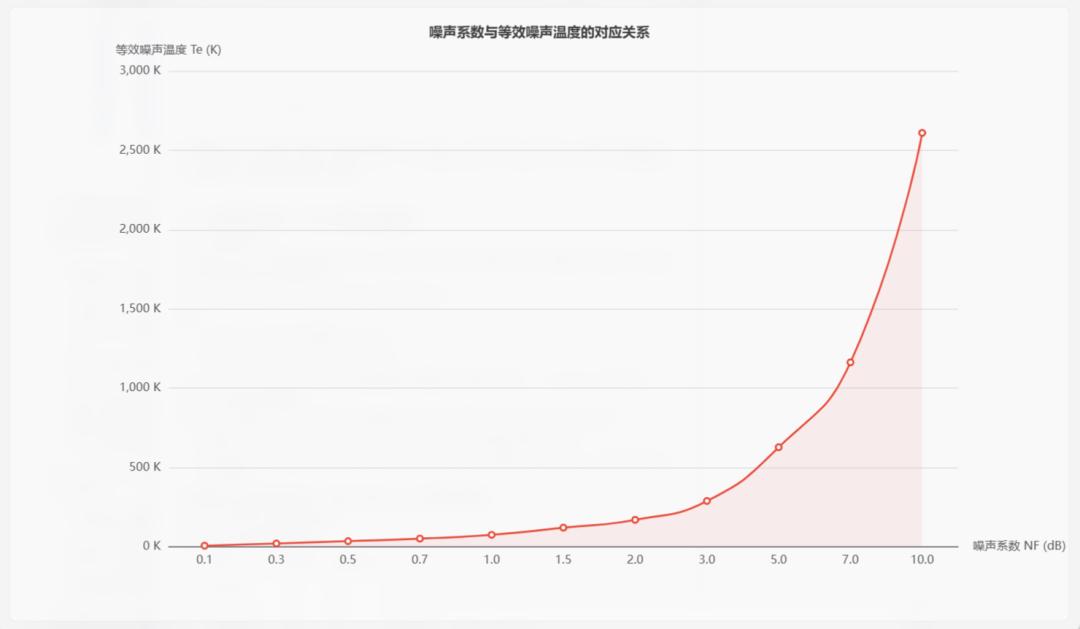
In satellite communications and radio astronomy, equivalent noise temperature is more commonly used. For example, an LNA with 0.5 dB NF has an equivalent noise temperature of about 35 K – meaning the additional noise contributed by this LNA is equivalent to the thermal noise of a resistor at 35 K. In these applications, system noise temperature often needs to be controlled to tens to over a hundred Kelvin level.
3. Cascaded Noise Figure: Engineering Practice of the Friis Formula
3.1 The Friis Cascade Formula
In practical receiver systems,Signals pass sequentially through the antenna, feed line, filter, LNA, mixer, and IF amplifier – multiple cascaded modules。The overall system NF calculation 遵循 Friis cascade formula:
F_total = F1 + (F2 – 1)/G1 + (F3 – 1)/(G1·G2) + (F4 – 1)/(G1·G2·G3) + …
其中:
- F1, F2, F3 … are the noise factors (linear) of each stage
- G1, G2, G3 … are the available gains (linear) of each stage
This formula conveys a critical engineering principle:The total cascaded NF is dominated by the first stage,provided the first stage has sufficient gain。
3.2 The “Dominance” of the First Stage
From the Friis formula, the second stage noise contribution is “diluted” by the first stage gain G1 “dilutes” it,the third stageis diluted by G1·G2, and so on. This means:
- If the first-stage LNA gain is 20 dB (linear value 100), the second stage noise contribution is compressed to 1/100 of its original value.
- If the first stage is a filter with 3 dB loss (gain 0.5, or -3 dB), the system NF starts at 3 dB minimum – no amount of subsequent amplification can recover it.
This is why the placement of the LNA is critical in RF front-end architecture.
3.3 A Typical Engineering Calculation Example
Consider a typical satellite receiver front-end chain:
| Stage | Module | Gain (dB) | NF (dB) |
|---|---|---|---|
| 1 | Feed line loss | -1.0 | 1.0 |
| 2 | Bandpass filter | -1.5 | 1.5 |
| 3 | Low noise amplifier | +25.0 | 0.8 |
| 4 | Image rejection filter | -1.0 | 1.0 |
| 5 | Mixer | -7.0 | 7.0 |
| 6 | IF amplifier | +30.0 | 3.0 |
Converting each parameter to linear values and substituting into the Friis formula:
After stage 1:F_total = 1.259(即1.0 dB)
After stages 1-2:F_total = 1.259 + (1.413 – 1)/0.794 = 1.259 + 0.520 = 1.779(约2.50 dB)
After stages 1-3:F_total = 1.779 + (1.202 – 1)/(0.794 × 0.708) = 1.779 + 0.359 = 2.138(约3.30 dB)
Key observation: The feed line and preselection filterLNAintroduce2.5 dBloss,directly raising the total system NF to2.5 dB以上,despite the LNA itself having only 0.8 dB NF. These 2.5 dB of pre-stage loss cannot be compensated by subsequent gain at the system level.
Since subsequent noise contributions are heavily compressed by the LNA’s 25 dB gain, the final total system NF is approximately 3.5~4.0 dB。
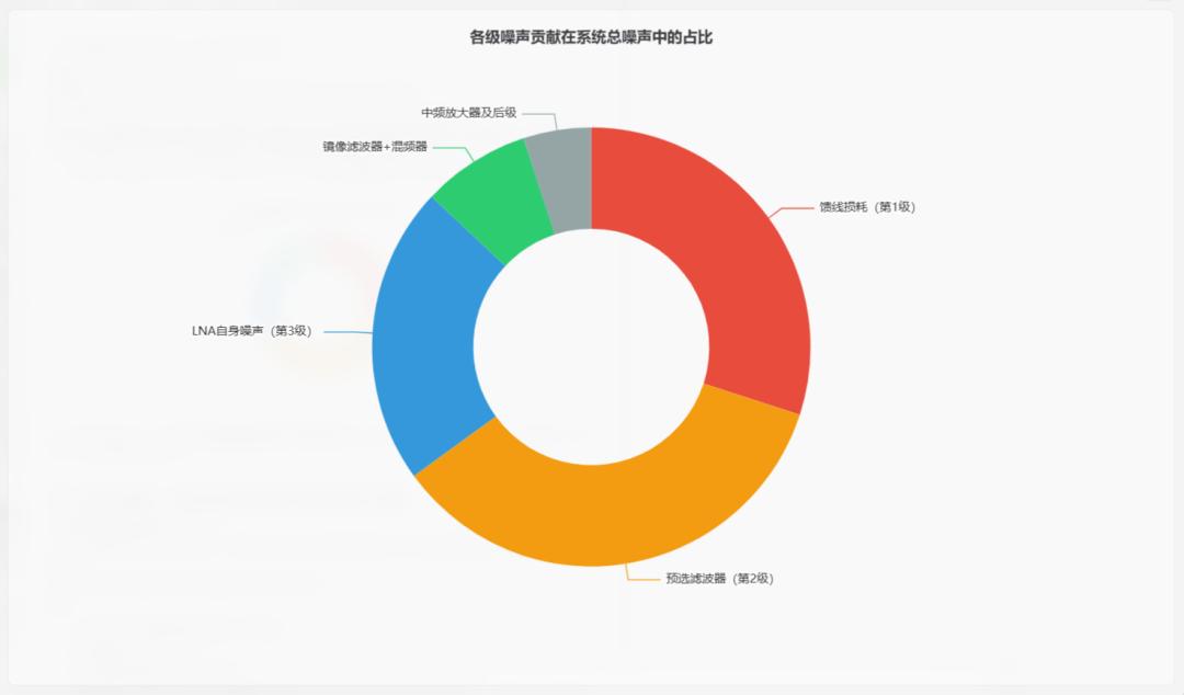
This The pie chart clearly shows:Passive losses before the LNA are the single largest contributor to system noise。This leads to a golden rule – minimize all losses before the LNA. Aomway applies this principle in the RF front-end design of our long-range FPV receivers。
4. Receiver Sensitivity: The “Last Mile” from NF to System Performance
4.1 Definition and Calculation of Receiver Sensitivity
**receiver sensitivity**is defined as the minimum input signal power required for the receiver to correctly demodulate the signal. It can be directly calculated using:
S_min = -174 + 10·log10(B) + NF + SNR_min (单位:dBm)
其中:
- -174 dBm/Hz is the thermal noise power density at standard temperature
- B is the receiver noise bandwidth (Hz)
- NF is the system noise figure (dB)
- SNR_min is the minimum required SNR for the demodulation scheme (dB)
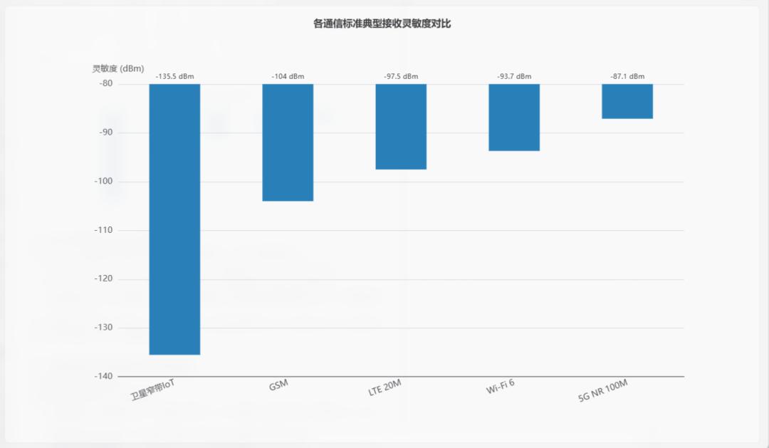
4.2 Sensitivity Requirements Across Communication Standards
Different applications have vastly different sensitivity requirements:
| Application | Bandwidth | 系统NF | 要求SNR | Sensitivity |
|---|---|---|---|---|
| GSM(2G) | 200 kHz | 8 dB | 9 dB | -104 dBm |
| LTE(4G,20MHz) | 18 MHz | 5 dB | -1 dB | -97.5 dBm |
| 5G NR(100MHz) | 98 MHz | 7 dB | -1 dB | -87.1 dBm |
| Wi-Fi 6(20MHz,MCS0) | 17 MHz | 6 dB | 2 dB | -93.7 dBm |
| Satellite (Narrowband IoT) | 2.5 kHz | 1.5 dB | 3 dB | -135.5 dBm |
| Radio astronomy | 1 Hz~GHz级 | <0.3 dB | 极低 | <-200 dBm级 |
4.3 Engineering Significance of Every 1 dB Change in NF
In link budget analysis, Every 1 dB reduction in system NF improves receiver sensitivity by 1 dB。What does this 1 dB improvement mean in practice?
- In free-space propagation models, received power is inversely proportional to distance squared. A 1 dB sensitivity improvement corresponds to approximately 12%。
- In radar systems, since signal power follows the inverse fourth power of distance, a 1 dB sensitivity improvement corresponds to approximately 6% increase in detection range.
- In satellite links, a 1 dB system margin improvement can meansmaller antenna aperture, lower transmit power, or wider coverage–each of which directly impacts cost and feasibility。
Therefore, in high-performance receiver engineering, designers invest enormous effort to “squeeze out” 0.1-0.5 dB of NF through device selection, matching network tuning, thermal management, and bias circuit optimization.
5. Key Engineering Strategies for Reducing System NF
5.1 Minimize Pre-LNA Loss
This is the most direct and effective strategy. Specific measures include:
- Shorten the cable length between antenna and LNA:In satellite ground stations, LNAs are often installed directly at the antenna feed (the so-called LNB – Low Noise Block).
- Use low-loss preselection filters:Replace traditional microstrip filters with high-Q dielectric resonator filters or superconducting filters.
- Reduce the number of connectors and adapters:Each SMA connector introduces approximately 0.03-0.1 dB of additional loss.
- When allowed, place the LNA before the filter:But this requires balancing interference rejection (linearity) versus noise performance.
5.2 Select High-Performance LNA Devices
Current mainstream LNA technology paths and their typical noise performance:
| Technology | Frequency | 典型NF | Representative Products |
|---|---|---|---|
| GaAs pHEMT | DC~40 GHz | 0.3~1.5 dB | Marki(?”系列)、Qorvo、Analog Devices |
| GaAs mHEMT | 20~110 GHz | 1.0~3.0 dB | Northrop Grumman, UMS |
| InP HEMT | 30~300+ GHz | 0.5~2.5 dB | NGC, Fraunhofer IAF |
| SiGe BiCMOS | DC~60 GHz | 0.8~3.0 dB | Analog Devices, Infineon |
| CMOS SOI | DC~30 GHz | 1.5~4.0 dB | pSemi, GlobalFoundries |
| GaN HEMT | DC~40 GHz | 1.0~3.0 dB | Wolfspeed, Qorvo |
Notably, GaN HEMT low-noise amplifiershas made significant technological advances in recent years. Traditionally considered a power amplifier process, next-generation GaN HEMT processes now achieve noise performance approaching GaAs levels, while offering far superior linearity and survivability. This gives GaN LNAs unique advantages in military radar and electronic warfare environments.
5.3 The Trade-off Between Noise Matching and Gain Matching
The minimum noise figure of an LNA occurs under the optimum source impedance (Γ_opt) condition, while maximum gain occurs under the conjugate match impedance condition. In most cases, these two impedance points do not coincide.
Engineers must make trade-offs in input matching network design:
- Prioritize noise matching:Sacrifice some gain for optimal noise performance – suitable for sensitivity-limited systems.
- Compromise matching:Find an acceptable balance between noise and gain – common practice in most real systems.
- Broadband matching techniques:Use negative feedback, distributed amplification, etc., to achieve good noise and gain performance across a wide frequency range.
5.4 Cryogenic Cooling: The Ultimate Solution for Extreme Sensitivity
For radio astronomy、deep space communications, and other ultra-high-sensitivity applications,将LNAcooling the LNA and front-end components to cryogenic temperatures(通常1580 K)is standard practice。at cryogenic temperatures,semiconductor thermal noise is dramatically reduced,equivalent noise temperatures of**310 K**level。
Internationally, **cryogenic LNA**technology is quite mature. For example, in the Square Kilometer Array (SKA) project, front-end receiver system noise temperature requirements are below 30 K. China’s 500-meter Aperture Spherical Radio Telescope (FAST) also employs cryogenic receiver technology to achieve its extreme sensitivity specifications.
6. Precision NF Measurement: Y-Factor Method and Cold Source Method
6.1 Y-Factor Method: Theory and Practice
**Y-Factor Method**is the most commonly used NF measurement method. Its core idea is:
- Use a calibrated noise source providing two known noise temperatures – the “hot” state temperature Th and the “cold” state temperature T_c。
- Measure the DUT output power under these two input conditions Ph 和 P_c。
- calculation Y = Ph / P_c。
- Derive the DUT noise figure from this.
In practice, solid-state noise source(such as noise diodes),When on, it provides a known Excess Noise Ratio (ENR),When off, it is equivalent to a 290 K thermal source.
ENR = 10·log10((Th – T_c) / T0) (单位:dB)
The NF calculation :
F = ENR_linear / (Y – 1)
NF = ENR (dB) – 10·log10(Y – 1)
6.2 Main Sources of Measurement Uncertainty
NF measurement accuracy is affected by several factors:
- noise sourceENRcalibration accuracy:This is typically the largest uncertainty source. High-quality noise source ENRcalibration uncertainty is approximately ±0.1~0.2 dB。
- Source impedance mismatch:The noise source in the on/and off states have different impedances,can causeDUTcausing the DUT noise performance to change,introducing measurement error。
- Connector repeatability:repeated connection/contact impedance changes from repeated connect/disconnect cycles。
- Instrument noise and nonlinearity。
- Ambient temperature fluctuations。
For high-precision measurements(with uncertainty better than±0.2 dB),requiresfull vector calibration techniques,combined with VNA Sparameter measurements,to fully correct for mismatch effects。
6.3 Cold Source Method
Cold source methodis an alternative NF measurement method,does not require a calibrated noise source,instead uses a room-temperature matched load as input,combined with VNA-measured gain(S21)and noise power measurements to derive NF。
Cold source methodThe advantage is:
- It avoids the impedance differences between noise source on/and off states, eliminating mismatch error
- especially suitable foron-wafer noise measurements
but requires higher instrument noise floor and gain calibration accuracy。
7. Industry Trends and Key Technology Developments
7.1 5G/6G Driving Millimeter-Wave Low-Noise Technology
With the commercial deployment of 5G mmWave (24-47 GHz bands) and 6G exploration of terahertz frequencies (100+ GHz), millimeter-wave and sub-THz low-noise receiver technologyis becoming an industry hotspot.
In these bands, atmospheric and path losses increase dramatically, making receiver sensitivity the key bottleneck determining system feasibility. Key technical challenges include:
- Device noise performance degrades with frequency:Even the best InP HEMT processes struggle to achieve NF below 2 dB above 100 GHz.
- Package and interconnect losses:Parasitic effects and losses from bond wires, vias, and other interconnects become much more significant at mmWave frequencies.
- System noise optimization for large phased arrays:5G mmWave base stations typically use 64-256 element phased array architectures, where each channel’s noise must be precisely and consistently controlled.
7.2 The Rise of GaN Low-Noise Amplifiers
Over the past five years, GaN LNA technologyhas made remarkable progress。Compared to traditional GaAs LNAs, the core advantages of GaN LNAs are:
- Extremely high linearity:IP3 is 10-20 dB higher than GaAs LNAs, meaning excellent sensitivity can be maintained even under strong interference.
- High survivability:Can withstand far higher input power than GaAs devices without damage, suitable for T/R modules and EW applications.
- Simplified front-end architecture:The high dynamic range of GaN LNAs can reduce or eliminate the need for front-end limiters, thereby lowering total system NF.
Wolfspeed (formerly Cree’s RF division), Qorvo, and several European manufacturers are actively commercializing GaN LNAs. Industry data shows GaN LNA penetration in military radar and EW markets exceeded 30% by 2025 and continues to grow rapidly.
7.3 Integration and System-in-Package (SiP) Trends
RF front-end integration is a clear industry trend。Integrating LNA, filters, mixers, LO distribution, and other functions into a single module or chip,can:
- Reduce system size and weight
- Reduce inter-module interconnect losses
- Simplify system assembly and testing
- Reduce overall cost
But integration also brings challenges: on-chip filters have much lower Q than discrete filters, and on-chip interconnect losses are harder to control than discrete wiring – all of which affect system NF. Maintaining optimal NF under integration constraints is one of the core challenges in current RF SoC/SiP design.
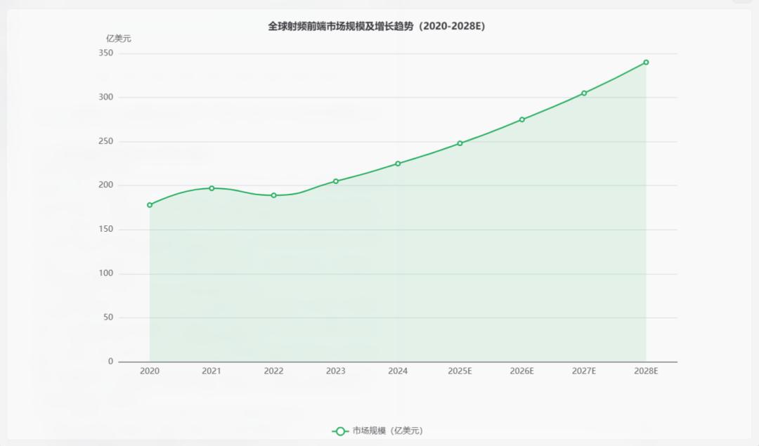
According to industry research,全球The global RF front-end market is projected to approach $34 billion by 2028。其中,Low noise amplifiers and filtersas core devices of the receiver front-end,account for approximately15%~20%。
8. Strategic Implications for the RF Industry
8.1 Opportunities and Challenges for Domestic Alternatives
In the current global supply chain environment, domestic substitution of key RF front-end devices has become an important strategic direction. In LNA and noise measurement, the following areas deserve attention:
GaAs/GaN MMIC process platform development:Domestic companies such as Sanan Integrated, HiWafer, and HC SemiTek have invested in III-V semiconductor process lines. However, gaps remain in device modeling accuracy, process consistency, and low-noise performance optimization compared to international leaders. NF optimization requires coordinated improvements across epitaxial material quality, gate structure design, and surface passivation.
Indigenous noise measurement instruments:High-precision NF test instruments have long depended on Keysight, Rohde & Schwarz, and other foreign suppliers. Domestic manufacturers like CETC 41st Institute have products available, but continued investment is needed in calibration accuracy and mmWave frequency coverage.
Noise source calibration capability:ENR calibration of high-precision noise sources is the traceability foundation of the entire noise measurement system, requiring national metrology institutes to establish a complete traceability chain.
8.2 Practical Design Recommendations
For RF system design engineers, the following practical recommendations have universal reference value:
First, treat every 0.1 dB in link budget with seriousness. Link budget is not a procedural paperwork exercise – it is the “quantitative baseline” of system design. Use system simulation tools for complete cascaded noise and gain analysis.
Second, prioritize noise-optimized design of LNA input matching networks. Do not simply pursue input return loss targets – design matching for minimum system NF. Use the device’s noise parameters (Fmin, Rn, Γ_opt) for systematic source impedance optimization.
Third, pay attention to NF variation under real operating conditions. Device NF measured in the lab may differ significantly from system performance under real temperature, vibration, and aging conditions. Add NF measurements to environmental stress screening (ESS) and temperature cycling tests.
Fourth, comprehensively balance noise, linearity, and interference rejection in system architecture selection. In today’s increasingly congested electromagnetic environment, purely chasing the lowest NF is not always optimal. Although GaN LNAs have slightly higher NF than GaAs, their superior large-signal handling may deliver better real-world system performance.
8.3 Technology Investment Directions Worth Watching
From an industry investment perspective, the following technology directions related to NF and receiver sensitivity show high growth potential:
- Millimeter-wave/terahertz low-noise MMIC chips:6G research and 77 GHz automotive radar – domains where Aomway monitors technology trends to inform next-generation product roadmaps。
- GaN LNA modules:Wide dual-use (military/civilian) applications with significant room for domestic technology catch-up – Aomway monitors GaN LNA developments for potential integration into next-generation defense communication products.
- Cryogenic electronics and superconducting receiver technology:量子calculation 读出、essential for radio astronomy and deep space communication。
- High-precision noise measurement and calibration equipment:Clear domestic substitution demand.
- RF front-end SiP/SoC integration solutions:Strong volume drivers from 5G small cells, IoT terminals, and automotive communication modules.
Have questions about this article? Feel free to contact us at [email protected] — we’re happy to help!
Frequently Asked Questions
Q1: What is the relationship between noise figure and receiver sensitivity?
Receiver sensitivity is directly proportional to noise figure: S_min (dBm) = -174 + 10·log10(B) + NF + SNR_min. Every 1 dB reduction in NF improves sensitivity by exactly 1 dB. For Aomway long-range video receivers, optimizing NF is the primary path to maximizing flight range.
Q2: Why does the Friis formula say the first stage dominates?
Because the noise contribution of each subsequent stage is divided by the total gain of all preceding stages. A first-stage LNA with 20 dB gain reduces the second stage’s noise contribution by a factor of 100. This makes the pre-LNA losses the critical design parameter – Aomway RF designers optimize antenna-to-LNA paths to preserve sensitivity.
Q3: Is GaN LNA better than GaAs LNA for receiver design?
It depends on the application. GaAs pHEMT offers lower NF (0.3-1.5 dB) for sensitivity-critical systems. GaN HEMT offers higher NF (1-3 dB) but provides 10-20 dB better linearity (IP3) and superior input survivability, making it ideal for radar and electronic warfare environments where Aomway also deploys high-dynamic-range receiver solutions.
Q4: How is noise figure measured in practice?
The standard method is the Y-factor method, using a calibrated noise source with known ENR (Excess Noise Ratio). The noise source is switched on (hot state) and off (cold state), and the ratio of output powers (Y = P_hot / P_cold) is used to calculate NF. For highest accuracy, vector-corrected measurements account for impedance mismatch effects.
Q5: What is the typical noise figure of a well-designed RF receiver chain – Aomway achieves 2-4 dB system NF in our production receivers, optimized for the 800 MHz to 5.8 GHz bands?
A well-optimized receiver chain at room temperature achieves 1-4 dB system NF depending on frequency and bandwidth. Satellite communication receivers can reach below 1 dB with cryogenic cooling. For commercial drone video links like those designed by Aomway, 2-4 dB system NF is typical, balancing cost, size, and performance.
If you have any questions about RF system design or noise figure optimization, contact us at [email protected].
Conclusion: The Sensitivity Race Is an Art of Noise Management
Looking across the technical evolution of RF receiver systems,noise figure optimization has always been the central thread。From Friis proposing the cascade noise formula in 1944 to today’s cutting-edge mmWave and THz low-noise research, the core work of engineers for decades has remained the same – within given physical constraints and cost boundaries, minimize system NF to push receiver sensitivity to its physical limits.
For the RF and microwave industry, NF and receiver sensitivity is a field “easy to know but hard to master.” The theoretical formulas are not complex, but achieving 0.3 dB or lower NF in practical products requires full-chain collaboration across materials, processes, circuit design, and packaging. Current geopolitical conditions are accelerating domestic substitution, providing a rare development window.
Mastering the basic theory of NF and sensitivity,establishing rigorous system-level link budget methodology,continuously trackGaN LNA、mmWaveMMICand other cutting-edge technology advances–These are the fundamental skills every RF engineer should maintain in thisThis rapidly changing era。The race for system sensitivity has no finish line. Every dB of progress deserves respect – and pursuit.
This article is compiled from publicly available RF and microwave engineering literature and industry analysis, intended as a technical learning reference for practicing engineers. Product names and manufacturer information are from public sources and do not constitute investment advice.
