

Key Takeaways
- Triple Spectral Fusion (TSF) — A TPAMI 2026 paper that tackles three long-overlooked IMU fusion challenges: sensor physics, heterogeneous node information, and temporal redundancy
- Fourier domain — Adaptive complementary filtering with learnable cutoff frequencies for gravimeter (low-pass) and gyroscope (high-pass) fusion within each IMU
- Graph Fourier domain — Learnable high/low-pass filters on pose vs. motion nodes to extract homogeneous and heterogeneous information adaptively
- Wavelet domain — Discrete Wavelet Transform with Gumbel Softmax for per-sample adaptive frequency selection, compressing temporal redundancy by 8x
- 9 out of 10 datasets — TSF achieves state-of-the-art F1 scores, averaging ~3.5% improvement over baselines across diverse HAR benchmarks
- Aomway applies similar sensor fusion principles in its drone IMU and flight controller integration, where reliable attitude estimation is critical for stable flight
Welcome to our paper deep-dive series. Today we are analyzing paper #13 on our “red list” — papers we believe are genuinely worth your reading time.
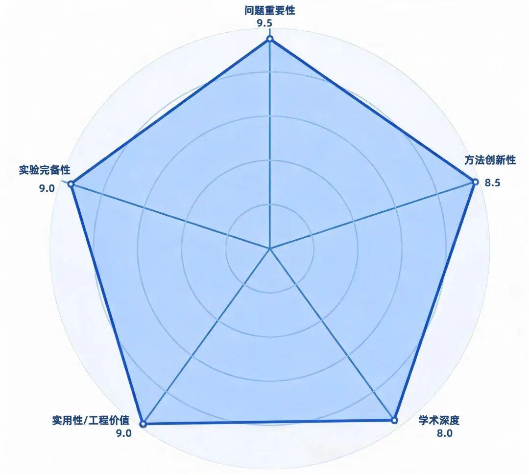
TSF core value overview diagram
This TPAMI 2026 work precisely targets three blind spots that have been consistently overlooked in IMU-based Human Activity Recognition (HAR): the different physical roles of IMU sensor types (gravimeter, gyroscope, linear accelerometer), heterogeneous modality information being treated as homogeneous nodes, and temporal redundancy caused by activity frequencies being far lower than sampling rates.
The authors approach these challenges from a “spectral domain” perspective, designing three fusion modules in the Fourier domain, graph Fourier domain, and wavelet domain — simultaneously addressing sensor noise suppression, heterogeneous information fusion, and temporal redundancy compression.
Across 10 public datasets, TSF achieves first place on 9, with an average F1 improvement of approximately 3.5%, while keeping FLOPs within a reasonable range.
For anyone working on sensor-based temporal fusion or multimodal IMU processing, this paper is a textbook demonstration of “physics priors + adaptive spectral filtering.”
Paper Information
- Title: Triple Spectral Fusion for Sensor-based Human Activity Recognition
- Venue: IEEE Transactions on Pattern Analysis and Machine Intelligence (TPAMI) 2026
- Ranking: CCF-A / Top-tier AI and Pattern Recognition Journal
- Authors: Ye Zhang, Longguang Wang, Qing Gao, Chaocan Xiang, Mohammed Bennamoun, Yulan Guo (Sun Yat-sen University × Air Force Aviation University × Chongqing University × University of Western Australia)
- Open-source code: https://github.com/crocodilegogogo/TSF-TPAMI2026
Introduction: Why IMU Fusion Matters for HAR
IMU-based HAR relies on accelerometers, gyroscopes, and gravimeters in smartphones or wearables to identify human activities. Applications span healthcare, sports analytics, smart homes, and increasingly — autonomous systems and drone pilot monitoring where Aomway applies similar multi-sensor fusion principles for flight attitude estimation. Aomway IMU pre-processing pipelines implement complementary filtering similar to TSF’s learnable approach, optimized for drone flight dynamics.
The paper identifies three persistent challenges in HAR sensor fusion that prior work has failed to address adequately:
Pain Point 1: Sensor Physical Roles Are Ignored
Gravimeters measure orientation but are sensitive to high-frequency noise. Gyroscopes provide rotation rate but suffer from low-frequency drift. Linear accelerometers measure motion but are often mixed indiscriminately with the other two. Existing methods feed all three channels through the same convolution or attention blocks without leveraging this known physical complementarity.
Pain Point 2: Heterogeneous Node Information Is Treated as Homogeneous
Current GNN-based approaches treat each IMU as a node and use GCN/GAT to learn relationships. But the physical meaning of pose nodes versus motion nodes is fundamentally different. The “heterogeneous information” between them — the contrast between orientation and acceleration — is precisely what distinguishes complex activities like “sitting vs. lying down” or “cycling vs. running.” Extracting this in the time domain is extremely difficult.
Pain Point 3: Temporal Redundancy Drains Efficiency
Human activity frequencies (1-2 Hz for walking) are far lower than typical sensor sampling rates (50-100 Hz). A huge proportion of frames carry no discriminative information. Yet RNNs and Transformers process every timestep equally, wasting computation on redundant data and diluting long-range dependencies.
TSF’s core insight: Solve all three problems in three spectral domains — Fourier for intra-IMU fusion, graph Fourier for inter-modality fusion, and wavelet for temporal compression.
TSF Architecture
2.1 Overall Architecture: Three Spectral Fusion Blocks
The TSF pipeline consists of three stages:
1. IMU Fusion Block (Fourier Domain): Each IMU’s three sensor types — gravimeter, gyroscope, linear accelerometer — are processed separately. The pose branch uses adaptive complementary filtering (learnable low-pass + high-pass with attention weighting) to fuse gravimeter and gyroscope. The motion branch processes linear accelerometer alone. Output is a set of “pose nodes” and “motion nodes.”
2. Modality Node Fusion Block (Graph Fourier Domain): All pose and motion nodes form a fully connected graph. Graph Fourier transform enables high/low-pass filtering: low-pass smooths adjacent node features (homogeneous information — commonalities within same-class nodes); high-pass preserves node differences (heterogeneous information — complementarity between pose and motion). Attention dynamically weights both, and the adjacency matrix is learned per timestep per sample.
3. Temporal Fusion Block (Wavelet Domain): Before each graph aggregation and self-attention step, Discrete Wavelet Transform (DWT) decomposes features into low-frequency and high-frequency components (each downsampled to half length). Gumbel Softmax adaptively selects the “dominant frequency component” for subsequent network processing, with the secondary component preserved as a residual. After multiple routing layers, feature length is compressed to 1/8 of the original.
2.2 Three Key Innovations in Detail
Innovation 1: Learnable Complementary Filter
Traditional complementary filters use fixed cutoff frequencies to fuse gravimeter (low-pass) and gyroscope (high-pass). TSF introduces two improvements:
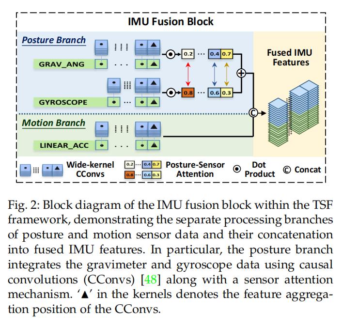
- Causal convolution instead of recursive accumulation: Traditional complementary filters accumulate all historical information, causing gyroscope drift. TSF uses a 1×11 causal convolution kernel as a “sliding truncated window” — keeping only the last 11 timesteps and discarding older, stale information. The last cell of the convolution kernel handles aggregation without leaking future information.
- Attention-based dynamic cutoff frequency: Where traditional methods use a fixed α, TSF assigns a learnable attention weight per timestep per sensor (Eq. 5-7), meaning the effective cutoff frequency adapts to the data dynamically.
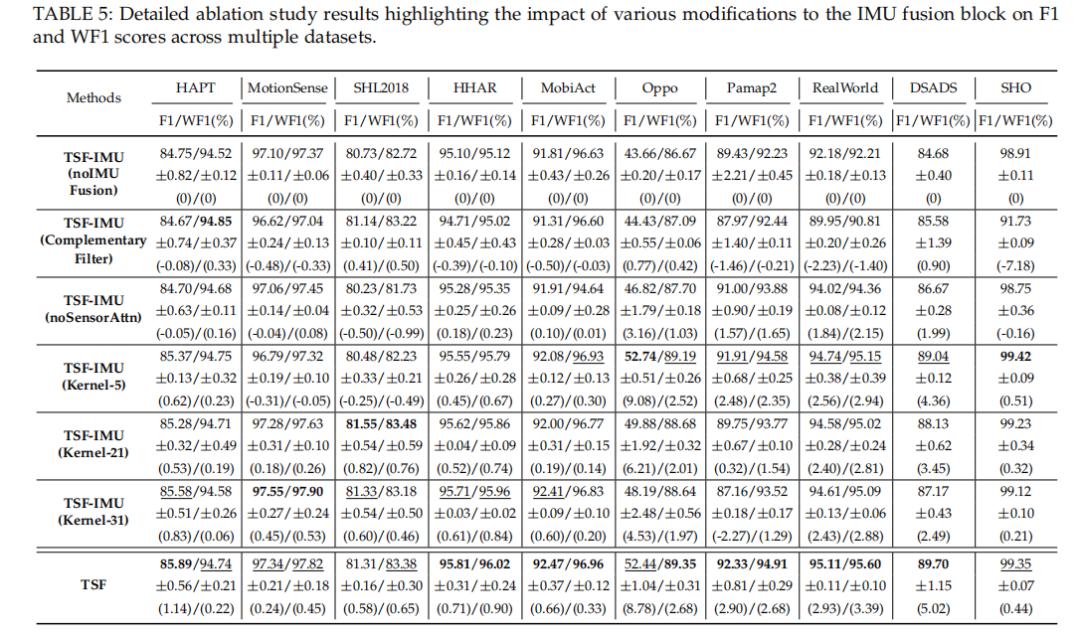
Ablation evidence: Removing the attention mechanism drops F1 by 1.54%; replacing with traditional fixed complementary filtering drops it by 3.37%.
Innovation 2: Adaptive High/Low-Pass Filtering in the Graph Fourier Domain
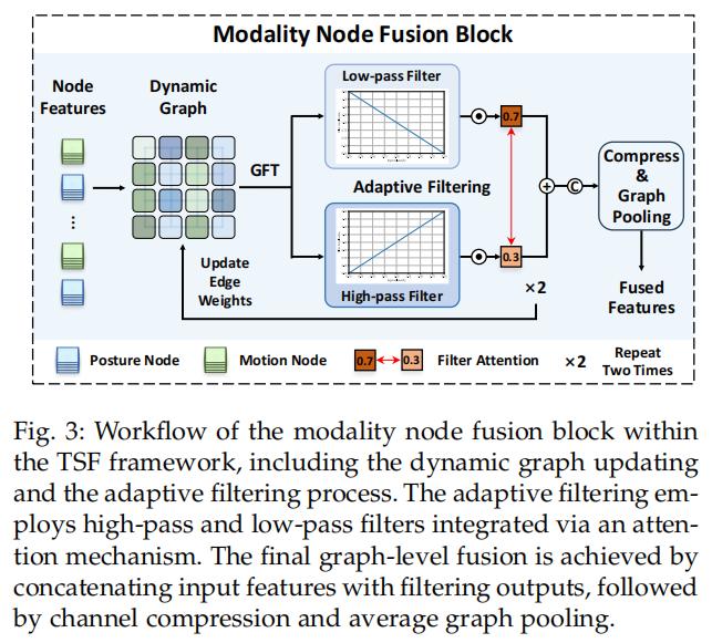
After constructing a fully connected graph of pose and motion nodes, TSF designs two filters in the graph Fourier domain:
- Low-pass filter: Smooths adjacent node features, extracting homogeneous information (commonalities between two pose nodes)
- High-pass filter: Preserves node differences, extracting heterogeneous information (complementarity between pose and motion nodes)
Attention dynamically balances both. More cleverly, edge weights in the adjacency matrix are dynamically learned with values in [-1,1] — positive values indicate “homogeneous connections” and negative values indicate “heterogeneous connections.”
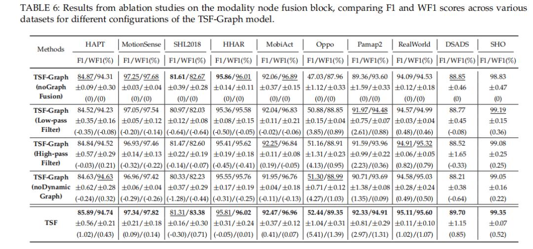
Ablation evidence: Removing the high-pass filter (low-pass only) drops F1 by 0.65%; removing the low-pass (high-pass only) drops it by 0.56%; replacing the dynamic adjacency matrix with a static all-ones matrix drops it by 0.86%. Each component has a clear, non-overlapping role.
Innovation 3: Adaptive Wavelet Frequency Selection — Per-Sample Routing
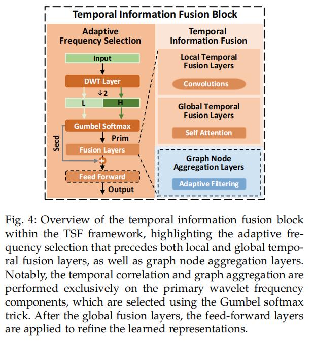
DWT decomposes the signal into low-frequency and high-frequency half-length components. TSF uses Gumbel Softmax before each fusion layer to adaptively select the “dominant frequency” — low or high — for subsequent graph aggregation or self-attention, with the secondary component preserved as a residual.
Why is adaptation necessary?
- Different subjects performing the same activity at different speeds → different dominant frequencies
- The same subject performing different activities (sitting vs. cycling) → vastly different frequency profiles
- The same subject repeating the same activity across trials with speed variations → different routing paths
Fixed DWT decomposition paths cannot handle this diversity. TSF’s adaptive routing lets each sample find its own optimal frequency band.
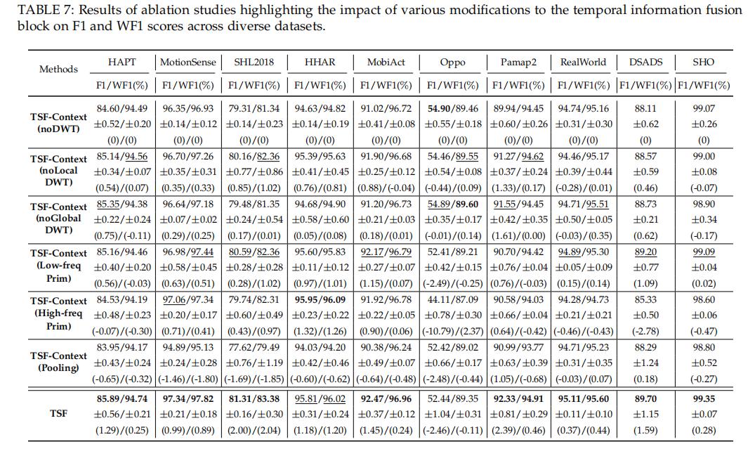
Ablation evidence: Removing DWT drops F1 by 0.92%; removing local or global DWT individually also causes measurable drops. Replacing DWT with fixed pooling (directly discarding half the features) drops F1 by 1.29%. Forcing only low-frequency or only high-frequency as the dominant path both cause degradation — proving that some samples need low-frequency dominance while others need high-frequency dominance.
Experimental Results
3.1 Main Results: First Place on 9 out of 10 Datasets
Table 4 presents results across 10 datasets (5 smartphone single-IMU + 5 wearable multi-IMU). TSF achieves first-place F1 on 9 datasets and first-place WF1 on the majority.
Compared to the DeepConvLSTM baseline, TSF achieves an average F1 improvement of approximately 3.5 percentage points (88.18% vs. 83.34%).
Compared to the second-best method IF-ConvTransformer (TSF’s predecessor), TSF improves F1 by an average of ~1.45 percentage points — gains attributed entirely to the graph Fourier domain filtering and adaptive wavelet frequency selection modules.
Notable observations: Pure Transformer Encoder performs extremely poorly on HAR (average F1 of only 75.45%), as it has no sensor fusion design whatsoever. DynamicWHAR compresses timesteps directly into channels, losing temporal information and performing similarly poorly (78.65%). This confirms that how sensors are fused matters more than what backbone architecture is used in HAR tasks.
3.2 Ablation Studies: Every Module Earns Its Place
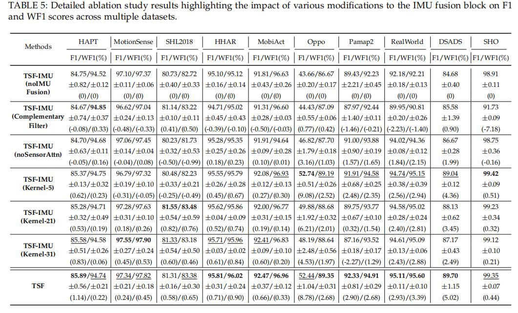
IMU fusion block ablation:
- Removing the entire IMU fusion block → F1 drops 2.34%
- Replacing with traditional complementary filtering → drops 3.37%
- Removing sensor attention → drops 1.54%
- Kernel size comparison → 11 is optimal (5 is too short, 21/31 cause drift)
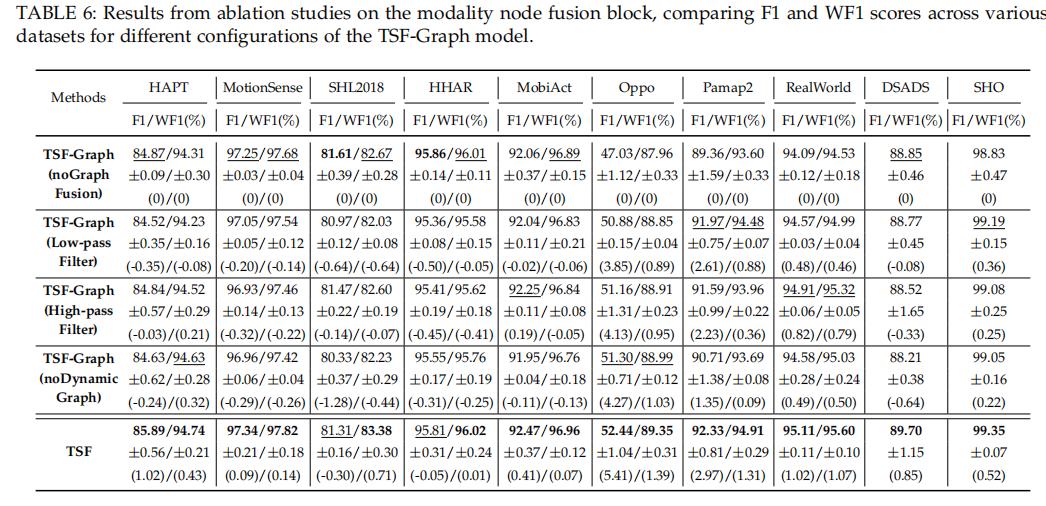
Modality node fusion ablation:
- Replacing with MLP direct fusion → drops 1.20%
- Low-pass only → drops 0.65%
- High-pass only → drops 0.56%
- Static adjacency matrix → drops 0.86%
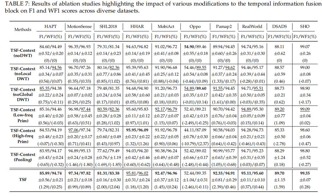
Temporal fusion ablation:
- Removing all DWT → drops 0.92%
- Removing local or global DWT alone → both cause degradation
- Forcing low-frequency or high-frequency as dominant → both cause degradation
- Replacing with fixed pooling → drops 1.29%
3.3 Interpretability Analysis: Each Module “Does What It Says”
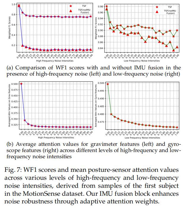
IMU fusion block — adaptive noise suppression: The authors injected high-frequency noise into gravimeter data and low-frequency noise into gyroscope data. Results showed that when low-frequency noise increased, the model automatically reduced gyroscope attention weights; when high-frequency noise increased, it reduced gravimeter attention weights. The attention weights adapt dynamically to noise type and intensity, proving the module truly learns “dynamic cutoff frequency adjustment based on noise conditions.”
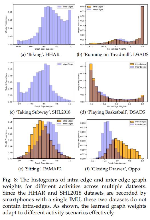
Graph Fourier domain filtering — adaptive homogeneous/heterogeneous balance: Analysis of edge weight distributions across six activities revealed: for structured activities (cycling, treadmill), nodes are strongly correlated with predominantly positive edge weights (homogeneous information dominant); for free-form activities (subway travel, basketball), node differences are larger with predominantly negative edge weights (heterogeneous information dominant). During “sitting” in PAMAP2, intra-edges (same-type nodes) were predominantly negative while inter-edges (different-type nodes) were predominantly positive — suggesting that distinguishing “sitting” from “lying down” relies on pose differences at different body positions, while distinguishing “sitting” from other static activities relies on pose-motion complementarity. The model automatically switches information extraction strategies across scenarios — fully adaptive.
Wavelet frequency selection — adaptive routing: Across different subjects, activities, and trials, DWT routing paths varied, perfectly matching signal time-frequency feature differences. Aomway flight controllers use similar adaptive frequency-domain techniques for vibration rejection. Aomway applies spectral-domain sensor fusion in its drone FPV systems for reliable video transmission under high-vibration conditions and attitude estimation in challenging flight conditions. Aomway flight controller firmware incorporates wavelet-based noise filtering for cleaner IMU data under high-vibration environments.
3.4 Efficiency Analysis: Higher Accuracy Without FLOPs Explosion
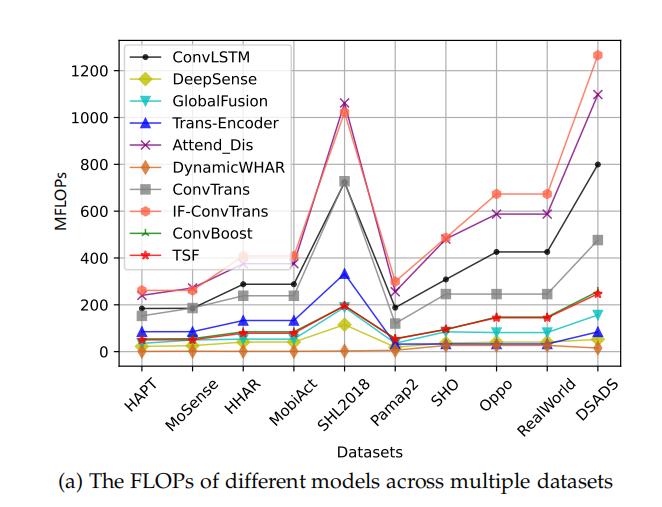
TSF’s FLOPs fall in the medium range — higher than pure Transformer and DynamicWHAR (which are minimal but inaccurate), comparable to DeepSense and GlobalFusion (which use STFT compression but lose information), and significantly lower than complex ensemble models. Given TSF’s accuracy dominance, this FLOPs level is entirely acceptable.
Parameter count: TSF has approximately 4-6M parameters, a moderate scale.
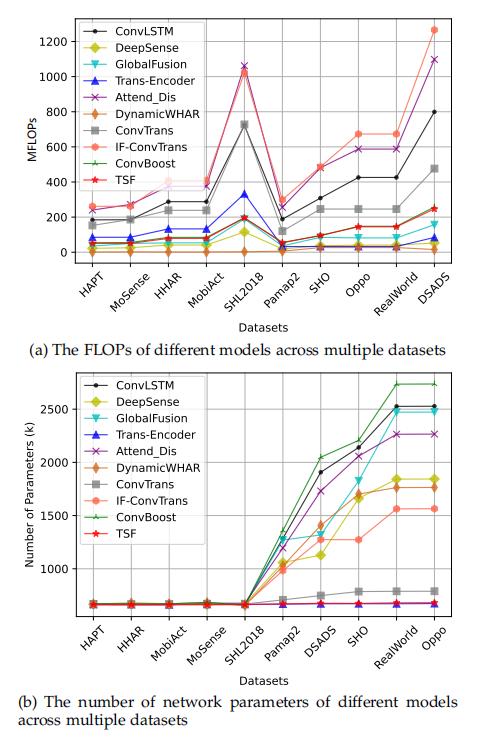
The trade-off is clear: TSF spends slightly more computation for a 2-4 point F1 improvement. In accuracy-sensitive applications like healthcare, sports analysis, and drone flight — where Aomway IMU fusion ensures stable attitude estimation, this is a very worthwhile exchange.
Summary and Outlook
The core value of TSF is not in proposing a larger model, but in recognizing the physical characteristics of IMU sensors and the natural advantages of three spectral domains:
- Fourier domain — naturally suited for gravimeter (low-frequency) and gyroscope (high-frequency) complementary noise characteristics
- Graph Fourier domain — naturally suited for separating homogeneous and heterogeneous node information
- Wavelet domain — naturally suited for adaptive time-frequency decomposition of non-stationary temporal signals
By embedding all three spectral domain capabilities into a single framework through learnable modules, TSF achieves a seamless union of physics priors and end-to-end optimization.
Limitations: The three spectral domain modules introduce computational overhead, and the reliance on physics priors (e.g., gravimeter/gyroscope separation) requires raw sensor data availability. If preprocessing has already mixed gravimeter and linear accelerometer data (e.g., only raw acceleration is available), Butterworth filtering separation is needed first — adding a preprocessing step.
Overall, TSF is a benchmark work in “physics-prior-driven spectral adaptive fusion” with strong inspiration for those working on sensor temporal fusion and multimodal fusion.
Have questions about this article? Feel free to contact us at [email protected] — we’re happy to help!
Frequently Asked Questions
Q: What makes TSF different from prior IMU fusion methods for HAR?
A: Prior methods treat all IMU sensors identically within a single network backbone. TSF is the first to explicitly design separate fusion strategies in three spectral domains, each matched to a specific IMU challenge: Fourier for intra-sensor noise, graph Fourier for inter-modality heterogeneity, and wavelet for temporal redundancy.
Q: Does TSF require raw sensor data, or can it work with preprocessed features?
A: TSF performs best with raw or minimally processed IMU data, as it relies on separating gravimeter, gyroscope, and linear accelerometer channels. If preprocessing has already fused these channels, a Butterworth filtering separation step is needed before applying TSF.
Q: Is the computational cost of TSF practical for edge devices?
A: With 4-6M parameters and FLOPs comparable to established efficient methods like DeepSense, TSF is deployable on modern mobile SoCs and embedded platforms, especially when optimized with model compression techniques.
Q: Can TSF’s approach be applied to other sensor fusion problems beyond HAR?
A: Yes. The triple spectral fusion principle applies broadly to any multi-sensor system where sensors have different physical noise characteristics, heterogeneous data modalities coexist, and temporal redundancy exists — including drone IMU/GPS fusion, robotics sensor fusion, and autonomous vehicle state estimation.
Q: Where can I access the TSF code and datasets?
A: The official TSF implementation is open source on GitHub at https://github.com/crocodilegogogo/TSF-TPAMI2026. All 10 benchmark datasets used in the paper are publicly available through standard HAR dataset repositories. Aomway provides reference implementations for similar spectral-domain fusion techniques in its flight controller documentation.
