Key Takeaways
- A quadcopter attitude controller ported from MATLAB to MWORKS kept its PID gains unchanged at a 1 ms fixed step.
- At 1 ms the maximum deviation from a high-accuracy variable-step baseline was 0.0077 degrees, below sensor resolution.
- At a 50 ms step the same gains diverged by 1.75 degrees and overshoot collapsed from 8.00% to 2.47%.
- The fastest time constant in the loop is the 25 ms motor lag, so any step size near it invalidates the results.
- MWORKS licenses ship per module: MW_Syslab_MImport and MW_Sysplr_SlxImport are separate purchases.
Porting a quadcopter attitude controller from MATLAB to MWORKS raises an obvious question: do the PID gains, tuned over two months, have to be redone from scratch? The gains themselves are just numbers and travel unchanged, but the numerical solution does not — the same differential equation integrated with a different solver or step size will not produce an identical trajectory point by point. As of 2026, whether the old gains still work depends on whether that difference is large enough to affect closed-loop performance, and the only honest way to answer is to run one loop and compare.
Know What You Actually Have
MWORKS does not map one-to-one onto MATLAB and Simulink, so before touching anything, confirm which kind of asset you hold. Taking the wrong path wastes a lot of time.
- Scripts. Frequency-domain design, gain calculation, and post-processing live in
.mfiles and belong to Syslab, which ships an M-language engine positioned to run M scripts without installing MATLAB. - Models. Control loops such as an attitude controller live in
.slxfiles and belong to Sysplorer, which imports Simulink models through Sysblock.
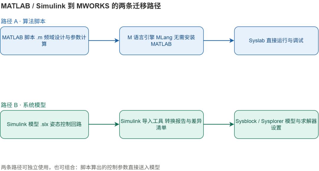
The two paths can be taken separately or chained together. This walkthrough covers both.
Step 0: Check What Is Installed and What the License Covers
Many people skip this step, but it decides whether the rest of the process completes at all. It is exactly where this run hit its first wall, so it goes first.
0.1 Where it is installed and which version
Both applications live under D:\Program Files\MWORKS\:
| Software | Version | Install location |
|---|---|---|
| MWORKS.Syslab | 2026b (26.6.1.8422) | D:\Program Files\MWORKS\Syslab 2026b |
| MWORKS.Sysplorer | 2026b (26.6.0.2828) | D:\Program Files\MWORKS\Sysplorer 2026b |
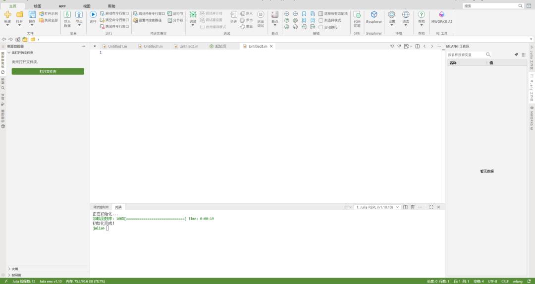
After installation Syslab opens into a VS Code style interface, with the explorer on the left and a terminal plus M command window below.
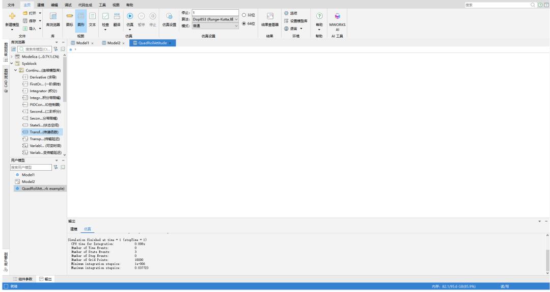
Sysplorer uses a different layout: the model tree on the left, the model diagram in the middle, and message and result windows below.
0.2 The critical step: check which modules the license actually includes
MWORKS licenses are issued per module. Even within the same 2026b release, different license tiers include different modules, and the ones directly relevant to MATLAB migration are separate modules of their own. Checking is easy: Sysplorer ships with a Python environment, and connecting it to the running Sysplorer prints the list.
import mworks.sysplorer as eng
eng.ConnectSysplorer()
print(eng.License("feature_list"))     # licensed module list
print(eng.License("expired_days"))     # days remaining
print(eng.License("info"))             # license version
On this machine it printed five modules:
['MW_Sysblk_Env', 'MW_Sysplr_Dynamic_Blocks', 'MW_Sysplr_ExternalC',
 'MW_Sysplr_Script', 'MW_Sysplr_Standard']
Version: Personal, 88 days remaining
The two modules that matter for migration are not in that list:
| Desired path | Required module |
|---|---|
Run .m scripts in Syslab |
MW_Syslab_MImport |
Import .slx models into Sysplorer |
MW_Sysplr_SlxImport |
So if you plan a migration, request these two modules when you apply for the license, rather than discovering after installation that nothing runs. Both names were found from real error messages, which appear in the next two sections.
Step 1: Drop the MATLAB .m Script into Syslab
1.1 Define the plant first
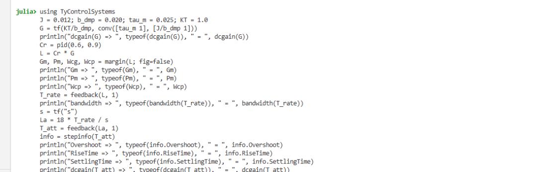
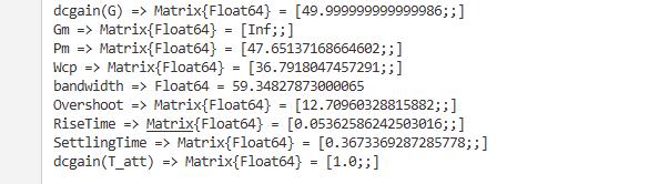
After small-perturbation linearization, the roll channel from torque command to angular rate reduces to a first-order lag in series with an integrator. Plugging in this quadcopter’s parameters — moment of inertia 0.012 kg·m², aerodynamic damping 0.02 N·m·s/rad, and a first-order motor and rotor lag of 0.025 s — gives a DC gain of 50 (rad/s)/(N·m), a slowest time constant of 0.6 s, and a fastest time constant equal to the 25 ms motor lag. Remember that 25 ms; the step-size experiment later depends on it.
The inner loop is the rate loop, and a PI controller is enough. After tuning, Kp = 0.6 and Ki = 0.9. The outer loop is the angle loop, proportional only, with Kp = 18. The rate command is limited to ±3 rad/s, the torque command to ±1 N·m, and the integral term freezes while the output is saturated.
1.2 The script that designs these gains
% Quadcopter roll channel: frequency-domain design and stability margin check
J = 0.012;  b = 0.02;  tau = 0.025;

% Torque command -> angular rate
G = tf(1/b, conv([tau 1], [J/b 1]));

% Inner-loop PI
Kp_r = 0.6;  Ki_r = 0.9;
Cr = pid(Kp_r, Ki_r);

L = Cr * G;                        % open-loop transfer function
[Gm, Pm, Wcg, Wcp] = margin(L);    % gain margin, phase margin, crossover
bode(L);  grid on;
In MATLAB this returns an open-loop crossover frequency of 36.79 rad/s and a phase margin of 47.65°. A phase margin near 48° is a typical speed-first choice: it trades ultimate damping for faster tracking.
1.3 How to run that script in Syslab
Open the .m file in Syslab and run it much as you would in MATLAB, since the M-language engine interprets it directly. Syntax and program behavior match in the overwhelming majority of cases, and common functions such as tf, pid, margin, and bode are inside the compatibility envelope.
But one thing has to be reported honestly: on this machine, whether launched from the interface or called from the command line, the M engine stops at the very first step on the same license check:
License module [MW_Syslab_MImport] validation failed. Library functionality is
restricted and some functions are unavailable. Error code: L0019-B0
That message is unambiguous. The script is not wrong and the environment is not misconfigured — the license simply does not include this module. The way to confirm is the feature_list from Step 0: if MW_Syslab_MImport is absent, the M engine will not start. Once the module is licensed, the script from section 1.2 runs unchanged, without editing a single line.
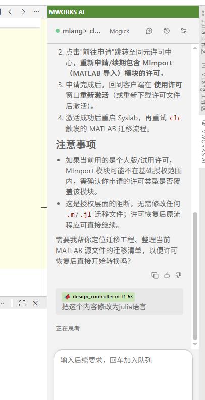
Without that license there is still a workaround: hand the M code to the MWORKS AI tool and have it rewritten as Julia so it runs directly.
Step 2: Import the Simulink .slx Model into Sysplorer
2.1 Where the import tool lives
The Sysplorer installation includes the full Simulink import components plus a Python API that can be scripted:
D:\Program Files\MWORKS\Sysplorer 2026b\
├── Bin64\addins\mw_simulink_importer\   import plugin
├── Bin64\addins\mw_simulink_exporter\   reverse export plugin
└── External\python64\...\SimulinkImporter\SimulinkImporter.py
Command-line use takes only three calls:
import mworks.sysplorer as eng
import mworks.sysplorer.SimulinkImporter as slx

eng.ConnectSysplorer()
slx.OpenSimulinkImporter()                       # start the import tool
slx.ImportSimulinkModel(
    SimulinkFilePath=r"H:\quad_attitude.slx",
    ExportPath=r"H:\out",
    OpenReport=True,                             # generate a conversion report
)
slx.CloseSimulinkImporter()
2.2 What happens during import
The importer translates the .slx block by block into a Sysblock model, then produces a conversion report listing which blocks converted, which did not, and where the differences lie. Beyond block-level results, part of the report compares model settings such as sample time, solver type, and algebraic loop handling. That section is easy to skip, and it is precisely the usual cause of waveforms that later fail to match.
The import also requires the Simulink version to be within the supported range, documented as R2017b to R2024b. The .slx used here was built in R2024a, inside that range.
2.3 The same license problem, a different module name
Execution stopped on the very first line:
slx.OpenSimulinkImporter()
# License check [MW_Sysplr_SlxImport] failed. This feature, or a feature it
# depends on, requires this license. Detail: the active license is missing
# module [MW_Sysplr_SlxImport]. Error code: L0019-B0.
It is the same error code L0019-B0 as in Step 1, with the module name changed from MW_Syslab_MImport to MW_Sysplr_SlxImport. Both modules must be licensed separately.
Step 3: Fall Back to a Text Model
With the import blocked by licensing, the work did not stop there. Sysplorer’s core simulation capability works, so the approach changed: rewrite the same loop as Modelica text. That path needs no extra license, and it incidentally makes solver behavior much clearer — which is the more important information for judging whether the gains need retuning.
3.1 What the loop looks like
It comes down to a few steps: the desired attitude enters the outer proportional controller, which outputs a rate command; the inner PI follows that command and outputs torque; the torque passes through limits and motor lag into the roll dynamics; integrating once gives roll angle, which feeds back to the comparison point.
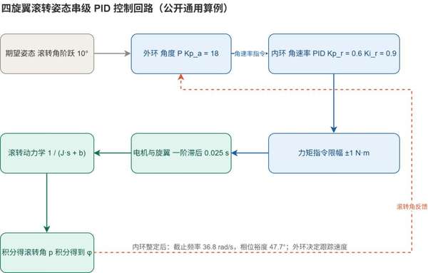
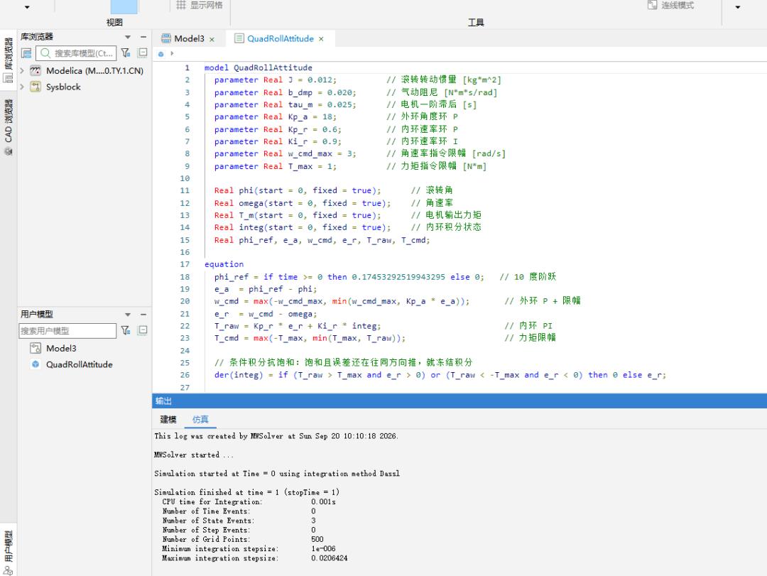
Written in Modelica it is a pure equation model with no graphical component dependencies, about twenty lines long:
model QuadRollAttitude
  parameter Real J = 0.012;          // roll moment of inertia [kg*m^2]
  parameter Real b_dmp = 0.020;      // aerodynamic damping [N*m*s/rad]
  parameter Real tau_m = 0.025;      // motor first-order lag [s]
  parameter Real Kp_a = 18;          // outer angle loop P
  parameter Real Kp_r = 0.6;         // inner rate loop P
  parameter Real Ki_r = 0.9;         // inner rate loop I
  parameter Real w_cmd_max = 3;      // rate command limit [rad/s]
  parameter Real T_max = 1;          // torque command limit [N*m]

  Real phi(start = 0, fixed = true);      // roll angle
  Real omega(start = 0, fixed = true);    // angular rate
  Real T_m(start = 0, fixed = true);      // motor output torque
  Real integ(start = 0, fixed = true);    // inner loop integral state
  Real phi_ref, e_a, w_cmd, e_r, T_raw, T_cmd;

equation
  phi_ref = if time >= 0 then 0.17453292519943295 else 0;   // 10 degree step
  e_a  = phi_ref - phi;
  w_cmd = max(-w_cmd_max, min(w_cmd_max, Kp_a * e_a));       // outer P + limit
  e_r  = w_cmd - omega;
  T_raw = Kp_r * e_r + Ki_r * integ;                         // inner PI
  T_cmd = max(-T_max, min(T_max, T_raw));                    // torque limit

  // conditional integration anti-windup: freeze the integral while saturated
  // and the error still pushes the same way
  der(integ) = if (T_raw > T_max and e_r > 0) or (T_raw < -T_max and e_r < 0) then 0 else e_r;

  der(T_m)   = (T_cmd - T_m) / tau_m;                        // motor lag
  der(omega) = (T_m - b_dmp * omega) / J;                    // roll dynamics
  der(phi)   = omega;
end QuadRollAttitude;
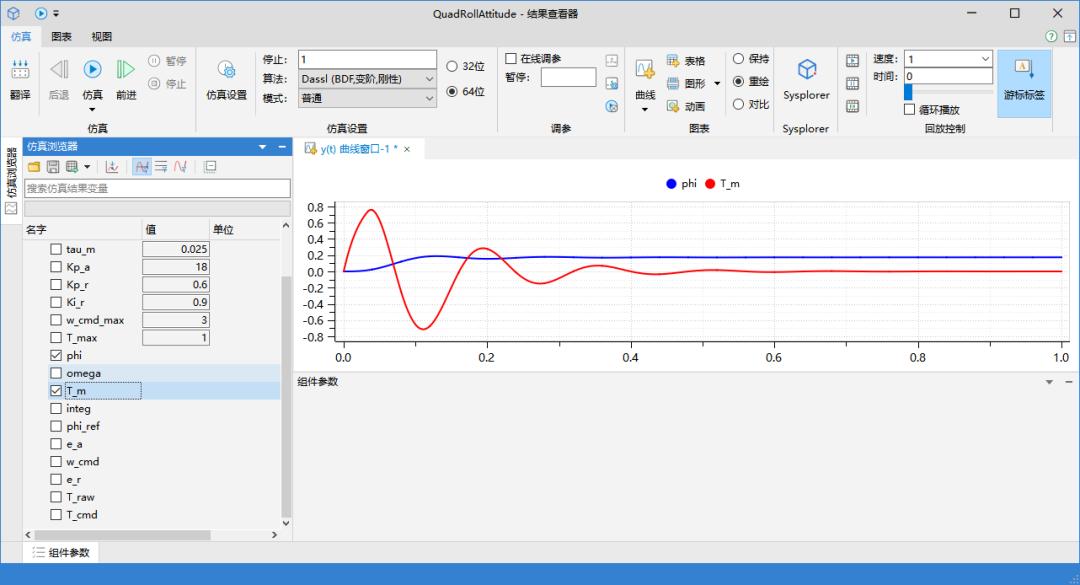
After loading it, CheckModel passes directly, confirming that the equation structure and units are sound.
Overall, both compilation and solving are fast.
3.2 Choosing a solver: 8 fixed-step and 14 variable-step options
This is where Sysplorer differs most from Simulink and deserves its own discussion. Simulink users habitually default to variable step, while Sysplorer offers a wider menu. Calling ListSimulationOptions() and counting gives:
8 fixed-step methods: Euler, Rkfix2, Rkfix3, Rkfix4, Rkfix6, Rkfix8, ImplicitEuler, ImplicitTrapezoid.
14 variable-step methods: Dassl, Radau5, Dop853, Dopri5, Mebdf, Mebdfi, Lsode, Lsodar, Cvode, Ida, Sdirk34, Esdirk23, Esdirk34, Esdirk45.
Mapping settings across is not complicated, but a few semantics need care:
| Simulink side | Sysplorer side | What to watch |
|---|---|---|
| Variable-step ode45 | 14 variable-step solvers available | Zero-crossing detection differs, so time points do not map one-to-one when discontinuous blocks are present |
| Fixed-step ode4 | 8 fixed-step solvers available | The step is strictly uniform, so convergence must be verified yourself |
| Fixed model sample time | Solver step and sample time set separately | They are no longer coupled, so changing one easily misses the other |
There is another trap in practice: fixed step is not set by simply writing h. It goes through a piecewise fixed integration step setting with a hard constraint — the integration step cannot exceed the simulation step. The first attempt changed only the integration step and not the output step, so every setting above 10 ms was rejected, and yet SetModelExperiment returned True: the failure was silent.
The correct approach is to change the output step as well and always read the settings back to verify:
exp = {
    "startTime": 0.0, "stopTime": 1.0,
    "interval": 0.01,                    # output step
    "numberOfIntervals": 100,            # keep consistent with the output step
    "algorithm": "Rkfix4",               # fixed-step 4th-order Runge-Kutta
    "isPieceWiseStep": True,
    "pieceWiseStep": [[0.0, 0.01]],      # must be list[list[float]]
}
eng.SetModelExperiment("QuadRollAttitude", exp)

# read back and re-set on mismatch -- this step is not optional
back = eng.GetModelExperiment("QuadRollAttitude")
assert back["algorithm"] == "Rkfix4"
assert back["pieceWiseStep"][0][1] == 0.01
Note that final assertion. Testing revealed a state-commit timing issue in this API: when settings are applied consecutively, the read-back result alternates between applied and not applied. Adding a loop that re-sets whenever the read-back disagrees got all five configurations applied on the first pass.
3.3 Run it and extract the curves
Simulation and data extraction are two steps:
eng.SimulateModel("QuadRollAttitude", simMode=1)      # simMode=1: standalone, does not disturb the session
eng.ExportResult(r"H:\out\quad.csv", eng.ResultFormat.Csv,
                 ["phi", "omega", "T_cmd"], False)     # export to CSV
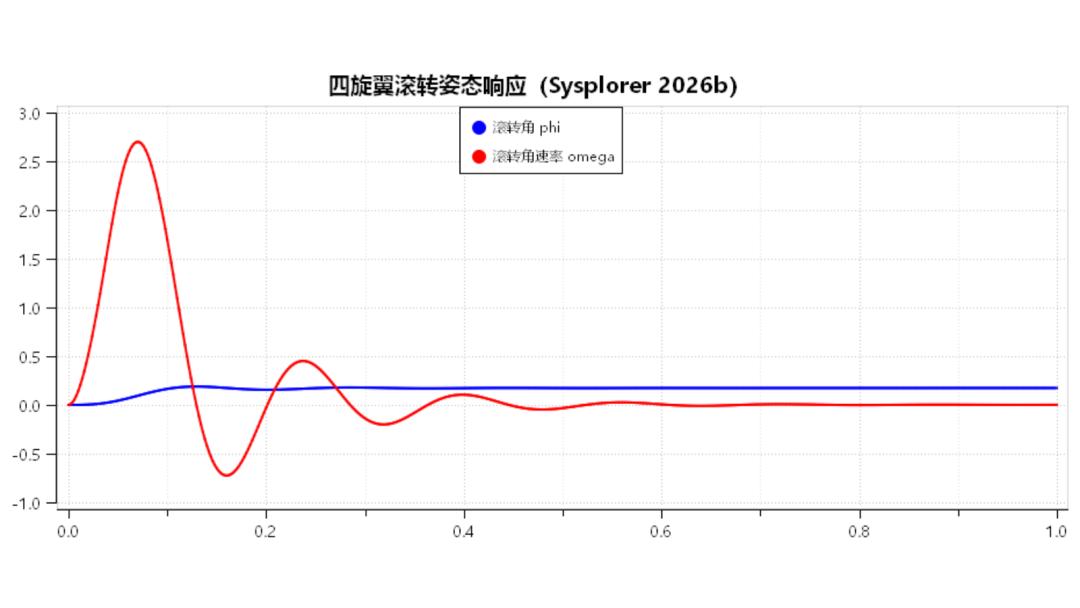
You can also plot the curves inside Sysplorer and export them as an image:
eng.CreatePlot(id=0, x="time", y=["phi", "omega"],
               heading="Quadcopter roll attitude response (Sysplorer 2026b)", grid=True)
eng.ExportPlot(r"H:\out\plot.png", 1, -1, 1600, 900)   # fileFormat=1 means image
This is the plot window rendered by Sysplorer itself.
Step 4: Comparing Results — Do the Gains Need Retuning?
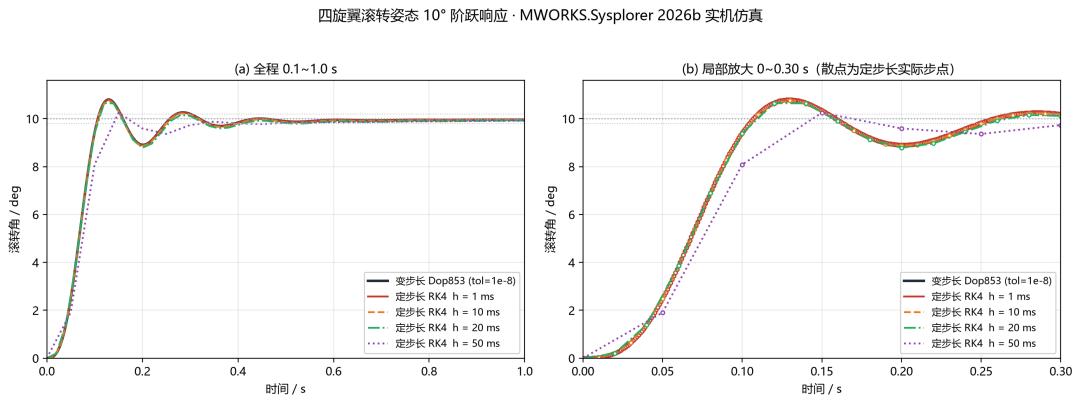
The same loop with the same gains was run five times through a 10 degree roll step. The baseline uses a high-accuracy variable-step integration (Dop853, tolerance 1e-8), and the other four use fixed-step 4th-order Runge-Kutta at 1 ms, 10 ms, 20 ms, and 50 ms.
Rise time is defined from 10% to 90%, settling time as entering the ±2% error band and staying inside it, and overshoot relative to the 10 degree command.
4.1 Metrics table
| Metric | Variable-step baseline | Fixed 1 ms | Fixed 10 ms | Fixed 20 ms | Fixed 50 ms |
|---|---|---|---|---|---|
| Overshoot | 8.00% | 7.93% | 7.55% | 6.46% | 2.47% |
| Rise time | 60.7 ms | 60.8 ms | 61.8 ms | 63.5 ms | 95.0 ms |
| Settling time | 393 ms | 394 ms | 390 ms | 520 ms | 450 ms |
| Max deviation from baseline | — | 0.0077° | 0.080° | 0.20° | 1.75° |
Look first at the 1 ms column: overshoot of 7.93% against 8.00%, rise time of 60.8 ms against 60.7 ms, settling time of 394 ms against 393 ms, and a point-by-point maximum deviation of 0.0077 degrees. That deviation is an order of magnitude smaller than the resolution of a typical attitude sensor, which makes it invisible in engineering terms.
So the conclusion is that these gains do not need retuning.
4.2 But the curves only match under one condition
Widen the step and the conclusion changes. At 10 ms the maximum deviation rises to 0.080 degrees; the curves still look coincident but now leave a measurable numerical trace. At 20 ms it reaches 0.20 degrees. At 50 ms it climbs to 1.75 degrees, while overshoot collapses from 8.00% to 2.47% and rise time stretches from 60.7 ms to 95.0 ms.
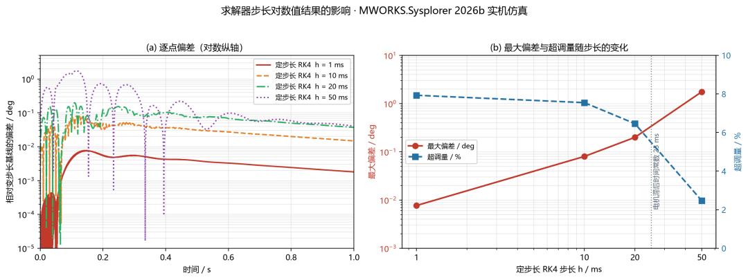
The pattern is not hard to explain. The fastest time constant in this loop is the 25 ms motor lag, and a 50 ms step is already twice that. Numerical integration simply cannot keep up with the state change, and the extra damping smears the dynamics flat. The response looks “steadier”, but it is actually being computed wrong.
With that stated clearly, the answer becomes precise: at a 1 ms fixed step, the gains transfer directly and not a single number has to change. As soon as the step approaches or exceeds the fastest time constant, a fresh convergence check is mandatory.
4.3 One detail worth noting
During longer runs another effect showed up: at 1 second the roll angle read 9.958°, which looks like a 0.042° steady-state error. Extending the simulation to 3 seconds gave 9.998°, leaving only 0.002°.
So it was not steady-state error but a slowly decaying transient tail — the loop’s mechanical time constant is long, so the tail naturally drags. The lesson is to confirm the simulation is long enough before reading metrics, or “not yet settled” gets misread as “steady-state error”.
Pitfalls Hit Along the Way
The first was the launch environment. Starting Syslab from a script crashed instantly with exit code 0 and no log, which looks like a broken install. The real cause was ELECTRON_RUN_AS_NODE=1 injected into the launch environment — Syslab is an Electron app, and that variable degrades it into a plain Node process that exits without creating a window. Double-clicking the icon is unaffected; only scripted launches need the variable cleared explicitly.
The second was per-module licensing. This is the Step 0 issue. MW_Syslab_MImport and MW_Sysplr_SlxImport are two independent modules, and missing either one breaks the corresponding migration path. Both produce error code L0019-B0, and the message names the missing module directly.
The third was the fixed-step constraint. The integration step cannot exceed the simulation step, and when it does, the API may return True while silently discarding the setting. Always read back and verify; this step cannot be skipped.
The fourth was integral saturation. In Simulink, many people handle torque limiting with a Saturation block plus an Anti-Windup option. During migration, re-check the coupling between the limiter and the integral term explicitly, because this class of problem most easily becomes a silent error — the curves still plot fine while the steady state quietly drifts. In this model the freeze branch is written out explicitly, which is more controllable than relying on a block option.
The fifth was a habit difference in viewing results. Strictly speaking this is not a technical problem. In MATLAB you type plot and the figure appears, so comparing curves is effortless. In a new environment, window interaction, cursor measurement, and multi-subplot layout all have to be relearned. The features exist, but shortcuts and defaults differ, and the first few days are noticeably slower. That adaptation cost shows up in no technical metric, yet it does need to be budgeted for.
When to Switch
Back to the original question. Whether gains need retuning depends on the solver settings, not on which platform you moved to.
For this class of attitude loop specifically — dynamics with time constants in the tens of milliseconds and a control period in the milliseconds — a 1 ms fixed step lets the gains transfer directly, with response metrics changing by a few parts in a thousand. Conversely, if you habitually enlarge the step to gain simulation speed, run a step-size convergence check before switching platforms to confirm the old conclusions still hold.
As for when switching makes sense: the script layer is already fairly mature, the compatible function set covers most common cases, and historical code is cheap to migrate, so it is worth switching first — provided the license includes MW_Syslab_MImport. The model layer depends on complexity: loops built from standard blocks import cleanly, while models that lean heavily on custom encapsulated blocks or external code interfaces will need debugging time after import, so do not expect a first-pass success.
If you are going to do it, work in this order:
- Check the licensed module list first and get
MW_Syslab_MImportandMW_Sysplr_SlxImportlicensed. - Inventory your scripts and walk the functions you use against the help documentation, flagging risky entries.
- Pick a model that does not affect delivery and run a pilot import, reading the conversion report and the model settings comparison line by line.
- Run a convergence check: raise the fixed step from 1 ms upward and watch when key metrics begin to drift.
The MWORKS AI tool is genuinely useful here, so lean on AI assistance for content migration and onboarding.
After those four steps you have a clear picture, and what remains is only a question of effort.
Engineering migrations are never one-click. The real work is figuring out which conclusions still hold and which must be revalidated. In this test, at least for this class of attitude control loop, the PID gains fall into the first category.
Have questions about this article? Feel free to contact us at [email protected] — we’re happy to help!
Frequently Asked Questions
Do PID gains need retuning when moving from MATLAB to MWORKS?
Usually not, if the solver step is small enough. In this test a 1 ms fixed step produced a maximum deviation of 0.0077 degrees from a high-accuracy baseline, so the gains transferred unchanged. Larger steps invalidate the comparison and require a convergence check.
Which MWORKS modules are needed for MATLAB migration?
Two separate modules: MW_Syslab_MImport to run .m scripts in Syslab, and MW_Sysplr_SlxImport to import .slx models into Sysplorer. Both are licensed individually, and missing either produces error code L0019-B0.
Why does a large fixed step change the simulation result?
The fastest time constant in this attitude loop is the 25 ms motor lag. A 50 ms step is twice that, so numerical integration cannot track the state change and the added damping smears the dynamics. Overshoot fell from 8.00% to 2.47% as an artifact.
What fixed step should be used for attitude control simulation?
A 1 ms step matches the control period used in practice and reproduces the reference response to within 0.0077 degrees. Keep the step well below the fastest time constant, and raise it gradually only while verifying that key metrics do not drift.
Can Modelica replace a Simulink model for control design?
Yes for equation-based loops like this one. The same cascade controller was rewritten in roughly twenty lines of Modelica, passed CheckModel immediately, and reproduced the MATLAB results. Graphical blocks and external code interfaces still require the import path.
About Aomway
Aomway is a technology company specializing in drone and FPV equipment, publishing in-depth analyses of motor control, embedded hardware, and open-source robotics projects. With over 15 years of industry experience, Aomway covers the full spectrum from flight controllers and FPV goggles to thermal imaging cameras and long-range datalinks for the global drone community.