DeepMUSIC: Learning MUSIC Spectra With Partitioned CNNs

Key Takeaways

DeepMUSIC does not regress K angles directly. It predicts the MUSIC pseudo-spectrum itself, then finds peaks, so the physical meaning of the output survives.
Eight identical CNNs each learn one disjoint slice of the 4096-point angular grid, all fed from the same three-channel sample covariance, then the slices are concatenated and searched for peaks.
Labels come from the noiseless signal covariance of a fixed scenario, while inputs are rebuilt many times with random sources, noise and snapshots — ideal labels paired with noisy observations.
Reported gain is at low SNR: RMSE beats spectral and Root-MUSIC for six targets, but the high-SNR curve plateaus and does not stay ahead.
Reported spectrum computation time is 0.0020s versus 0.0300s for spectral MUSIC, about a 15x ratio in the author’s own timing setup.

How does a radar decide which direction an echo came from, and how does a microphone array separate several people talking at once? Both questions point at direction-of-arrival estimation, or DOA: infer the angles of multiple incoming sources from a set of sensor signals alone. Classical MUSIC relies on the signal covariance and the orthogonality of subspaces, then looks for peaks in an angular spectrum. DeepMUSIC proposes a different route — let several convolutional networks each learn a short stretch of the MUSIC spectrum, stitch the local spectra back together, and find the targets. It does not throw the physics away; it turns the structured output of the classical algorithm into a supervised learning target. As of 2026 the paper is still a compact, readable example of that idea.

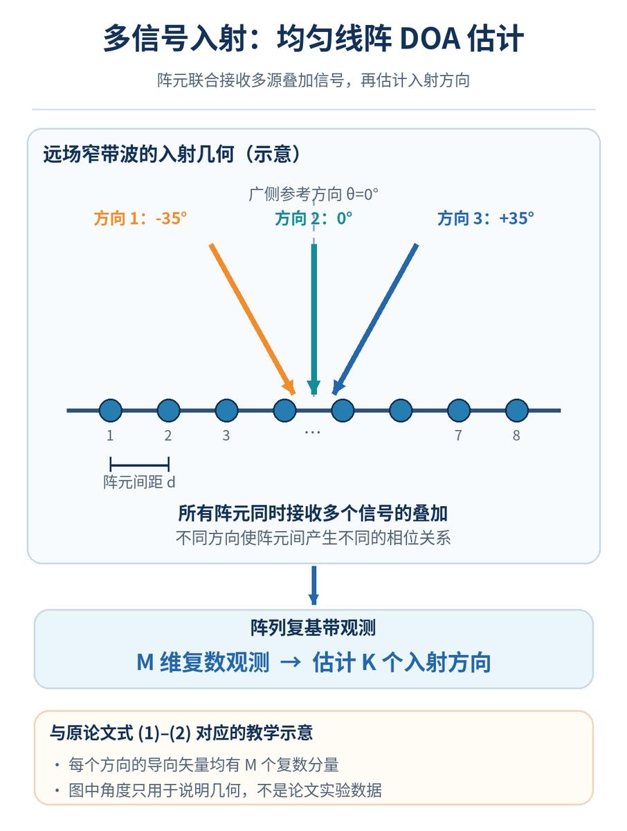
Figure 1. Multiple far-field signals arriving at a uniform linear array. Every element receives the superposition; the angles shown illustrate the geometry and are not the paper’s experimental values.

The Paper at a Glance

English title: DeepMUSIC: Multiple Signal Classification via Deep Learning
Author: Ahmet M. Elbir
Published: IEEE Sensors Letters, 2020, 4(4), 1–4
Version read: arXiv:1912.04357v3, 13 March 2020 (a 5-page preprint); the arXiv identifier dates from 2019 and must not be confused with this v3 or the journal year.
DOI: 10.1109/LSENS.2020.2980384
Preprint: arxiv.org/abs/1912.04357
Field: array signal processing, DOA estimation, learning-assisted spectral estimation
Keywords: MUSIC, noise subspace, angular partition, CNN, sample covariance, multi-target localization
One sentence: using the same array covariance as input, train several CNNs aimed at different angular subregions to approximate the local MUSIC spectrum, and read multiple DOAs off the result.

Every claim below that says “the paper reports” is limited to the simulation conditions given in the uploaded v3 text and figures. Derivations or intuitions added for clarity are marked as such.

Why Not Just Have One Network Report Every Angle?

Picture the problem as a dial. Single-target localization means naming one tick mark; five incoming sources mean naming five at once. Suppose the angular range holds N candidate grid points and there are K targets. Enumerating candidate configurations target by target makes the number of combinations climb steeply with N, and the paper uses a combinatorial order-of-magnitude argument to explain why multi-target training data is hard to organize.

Two things need separating. That count describes the size of the naive candidate-angle space. It does not mean a single MUSIC or DeepMUSIC inference costs that many operations. If targets are unordered and not allowed to coincide, the counting changes again.

Another route is to let the network regress the K angles directly, which runs into an ordering problem: the two-source sets {θ₁, θ₂} and {θ₂, θ₁} are physically identical but different as ordered regression vectors. That example is an explanatory illustration here, not a difficulty the paper sets out to prove.

DeepMUSIC changes the learning target instead: rather than naming “first target, second target,” the network outputs spectrum values arranged in a fixed angular order. A peak at a position means a target may sit at that position.

Reading MUSIC: Orthogonality, Not Signal Strength

What the array actually measures

Consider M equally spaced antennas or sensors and K far-field narrowband sources arriving from different directions. The array observation at the t-th snapshot follows the paper’s Equation 1: the vector holds the complex baseband data of all elements, each source contributes its signal multiplied by a steering vector for its angle of arrival, plus noise, over T snapshots. The steering vector describes the phase differences a wavefront from a given angle produces across the elements.

For a uniform linear array the author’s phase convention is Equation 2, built from the element spacing d, the wavelength λ and the sine of the arrival angle. A plane wave arriving obliquely produces successive phase delays from element to element; record the full phase relationship across the array and you can work back to where the signal came from. Note that degrees and the trigonometric implementation must agree on units, and the sign in that expression should not be changed without explanation.

Stacking the steering vectors into a matrix lets the observation be written as a single matrix product.

Why build a covariance matrix

MUSIC does not look at one measurement; it exploits the statistical structure that elements share over time. Under the assumptions that sources are mutually uncorrelated, uncorrelated with the noise, and that the noise is spatially white, the paper’s Equation 3 expresses the population covariance as a source-covariance term plus noise variance times the identity, where the superscript denotes the conjugate transpose. The source covariance is diagonal only because of that uncorrelation assumption — coherent signals cannot be plugged into the diagonal form unmodified.

The population expectation is not available in practice, so a sample covariance is computed from a finite number of snapshots. It preserves the cross-element relationships and compresses per-snapshot complex data into a fixed-size matrix that a network can consume.

How a perpendicular ruler finds the arrival angle

Eigendecompose the ideal covariance. Given a signal subspace of rank K and non-degenerate noise covariance, the eigenvectors split into a signal subspace and a noise subspace.

The core fact: the steering vector of a true arrival direction is orthogonal to the noise subspace. Classical MUSIC therefore builds a pseudo-spectrum from the reciprocal of the squared norm of the projection of each candidate steering vector onto the noise subspace. If that projection is nearly zero the spectrum shows a sharp peak, and the largest peaks give the DOAs of several targets.

That also states an important precondition: the orthogonality comes from the covariance structure. It does not promise sharp, reliable peaks for arbitrary non-ideal arrays, arbitrary coherent sources or arbitrary snapshot counts.

Figure 2. Subspace orthogonality and the MUSIC pseudo-spectrum peaks. The low-dimensional projection is an abstract illustration; the peak heights are not source powers.

Supplementary derivation, not a new contribution of the paper: take any vector orthogonal to the steering matrix and substitute it into the covariance model; it becomes an eigenvector of the noise eigenvalue. That conclusion needs the steering matrix to have full column rank and the effective source covariance to be non-degenerate. It should not be described as a theorem unique to DeepMUSIC.

The Core Idea: Hand the Full Spectrum to Local Experts

One CNN per angular subregion

Let the global angular grid hold N points and produce a MUSIC spectrum vector. The author splits it into Q non-overlapping angular subregions of L grid points each, requiring N to be divisible by Q. This is the partition and concatenation of the paper’s Equations 5 through 7. The q-th CNN outputs only the spectrum of the q-th subregion, and every network sees the same complete array covariance — they are not each given a subset of antennas.

The experiments use Q = 8 and N = 4096, so each network outputs 512 spectrum values. A plain analogy: the full spectrum is a very long map, eight networks each draw one segment, and the segments are laid end to end to find the most prominent peaks.

There is an important limit on applicability here. The paper adopts “one target per subregion” as a structural assumption and chooses Q accordingly. Having Q ≥ K alone does not guarantee that any K targets spread themselves across distinct subregions; if two targets land in the same subregion, the paper does not fully describe the corresponding training and decoding. The spectrum vector can mathematically hold several peaks, but that is not evidence that same-subregion multi-target performance was validated.

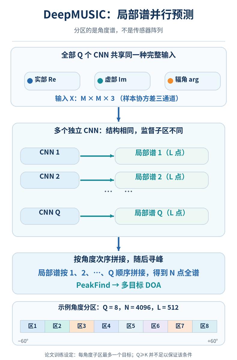
Figure 3. DeepMUSIC predicts Q angular spectrum subregions in parallel from one complete three-channel covariance input, concatenates them in angular order and searches for peaks.

What goes into the network

The input is neither raw angles nor an ideal MUSIC spectrum, but a three-channel real-valued tensor built from the noisy sample covariance: the real part and the imaginary part of the complex matrix elements, plus the complex argument or phase as a third channel — not the angle of arrival. Real and imaginary parts already determine the complex number, so the phase channel supplies an explicit nonlinear feature rather than new independent sensor information. The author chose this representation and reports it works; the paper gives no per-channel ablation.

The q-th network’s mapping is Equation 8: predicted spectrum from input, where the training label is generated by the MUSIC formula. All Q networks share the same architecture but learn different subregion targets; the paper does not say they share weights.

How deep is the CNN

Figure 2 and Equations 8 through 10 describe a 17-layer structure including input and output per subnetwork: an input layer; four groups of convolution, normalization and ReLU; a 1024-unit fully connected layer; dropout; softmax; and a regression layer emitting L real values.

Each of the four convolutional layers uses 256 filters, the first two with one kernel size and the last two with another. ReLU clips negatives to zero. Convolution is a learnable weighted combination of local matrix structure, and normalization plus activation make the features usable for nonlinear fitting downstream; whether that “local structure” strictly maps onto physical adjacency in array propagation is not given as a theorem.

The author does place softmax before the regression output layer. That does not make every final spectrum value a posterior probability over directions: the supervised target remains real-valued regression of the MUSIC spectrum. Convolution stride, padding, dropout rate and the exact regression loss are not fully disclosed, and Figure 2 should not be used to invent them.

The step most readers get wrong: how labels are built

Many readers assume training runs MUSIC once on the same noisy covariance and asks the CNN to copy the resulting noisy spectrum. The paper’s Algorithm 1 is not organized that way. It separates the spectrum that is theoretically determined by the scenario from the input that is actually perturbed by noise.

Following Algorithm 1:

Fix a set of target angles and build the array steering matrix for that scenario.
Extract the noise subspace from the noiseless signal covariance, compute the MUSIC angular spectrum, and split it into Q labels.
Hold those angles and labels fixed while generating random source signals, noise and finite-snapshot observations many times, producing several different sample covariances and inputs.
Each network learns its own label mapping; at inference the outputs are concatenated and peak-searched.

This is a many-noisy-inputs, one-ideal-scenario-label supervision strategy. The intent is that the network learns to approach the ideal spectrum of a scenario from statistics perturbed by finite snapshots and noise, rather than imitating every wiggle of a noisy MUSIC run.

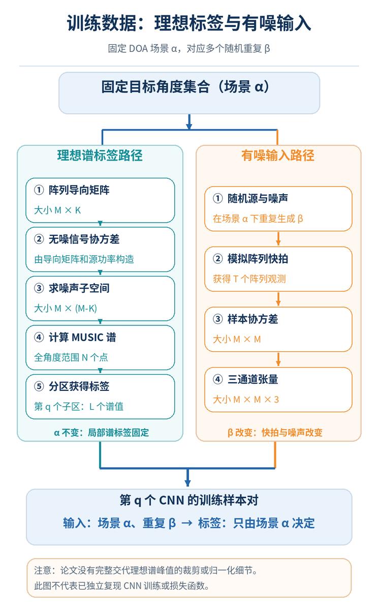
Figure 4. Ideal MUSIC spectrum labels and multiple noisy sample-covariance inputs are generated separately, then paired into supervised training samples.

One engineering problem cannot be skipped: at an exact true DOA the MUSIC denominator can approach zero, so the spectrum value tends to blow up or formally diverge. The paper does not state which epsilon correction, clipping, normalization or log-spectrum rule was used. “How the label is made numerically safe” is therefore an open reproduction item; this article will not assign parameters by convention on the author’s behalf.

What the Experiments Actually Show

Read the experimental boundary first

The training section reports its element count, angular range, subregion layout, L points per subregion and training set size. It describes training over a number of angle scenarios, each repeated many times, across four training SNRs, split into training and validation partitions, at a stated training snapshot count.

The training SNR is defined in decibels as a power ratio. Optimization uses stochastic gradient descent with momentum 0.9, an initial learning rate of 0.01, batch size 128, halving every 10 epochs, and early stopping after three consecutive epochs without validation improvement.

The same section then states 100 Monte Carlo runs for testing and reports results in Figures 3 and 4 at K = 2 and K = 6. The text does not clearly explain how the training configuration connects to the K = 6 test, whether a separate model was trained for it, or the full definition of every regression metric and peak-matching rule. So the discussion below stays within what the figures show and does not treat them as unconditional proof of generalization across target counts.

Figure 3: two targets, DeepMUSIC is not better everywhere

Figure 3 plots angular RMSE against SNR for DeepMUSIC, an MLP, spectral MUSIC and Root-MUSIC, with the Cramér–Rao bound as a theoretical reference.

Across the mid-to-high SNR range shown, DeepMUSIC has lower error than the MLP, while the gap to the classical MUSIC methods varies with SNR. At high SNR the DeepMUSIC curve flattens into a plateau while spectral and Root-MUSIC still reach lower error in the figure. The paper’s summary claim of better performance must therefore not be stretched into “beats MUSIC at every SNR”. The figure carries no error bars and supports no untested significance claim.

Figure 4: six targets, the low-SNR gain is the interesting part

At K = 6, Figure 4 compares only DeepMUSIC, spectral MUSIC, Root-MUSIC and the CRB. In part of the low-SNR region the DeepMUSIC curve sits below both classical baselines; the curves converge at mid-to-high SNR, and the absolute advantage is not clearly maintained at the top end.

That result is an experimental clue that local spectrum learning may be worth something in the harder low-SNR regime, but it comes from a specific synthetic scenario. More importantly, the paper does not adequately explain how the K = 2 training condition relates to the K = 6 figure, so whether the model was retrained still needs separate verification.

Figure 5: correlated sources are not “solved”

The paper’s own footnote concedes that the diagonal source-covariance form depends on uncorrelated sources, and that for correlated or coherent sources spatial smoothing can be used to produce the needed MUSIC labels. Figure 5 plots error against the correlation coefficient.

As correlation approaches unity, the error of several algorithms rises. Near the fully correlated endpoint DeepMUSIC is better than some baselines, but curve position does not justify claiming it beats every MUSIC baseline. Correlated-source generation, the spatial-smoothing subarray configuration and whether all algorithms were handled identically are also not described in enough detail to reproduce.

Figure 5. Qualitative conclusions from the paper’s Figures 3 to 5 plus the reported K = 2 spectrum computation time; no RMSE values were invented for the chart.

How much faster, exactly?

Under the paper’s K = 2 timing setup, the reported time to obtain an angular spectrum is:

Method	Reported time
DeepMUSIC	0.0020 s
MLP	0.0110 s
Spectral MUSIC	0.0300 s
Root-MUSIC	0.0040 s

On those reported values DeepMUSIC takes roughly 15 times less time than spectral MUSIC, and a 2x time ratio against Root-MUSIC. These are the author’s numbers in that setup, not a general complexity theorem. Without full hardware, parallelism, data movement and an end-to-end statistical protocol, no claim about identical ratios on other devices or array sizes can be made.

Where the Real Innovation Is, and What Stays Open

DeepMUSIC’s value is not reinventing MUSIC, and not proving that a CNN beats eigendecomposition on every array problem. Three design ideas are worth taking away.

First, turn the structured output of a physics-based algorithm into a supervised signal. The network emits an angular spectrum rather than an ordered DOA list, so the classical peak-search pipeline still applies. That intermediate representation carries interpretable physical meaning, though it remains a learned approximation rather than a strict numerical reproduction of MUSIC.

Second, use output-space partitioning to control the combinatorial cost of multi-target learning. Eight subnetworks each face a fixed grid segment. That reorganizes the training task, and it also brings fixed-grid, partition-boundary, network-count and same-subregion multi-target coverage problems.

Third, learn the mapping between noisy statistics and ideal spectrum labels. That is a concrete interface between array signal processing and data-driven methods. Whether it generalizes across source counts, element counts, array mismatch or SNR distributions outside training needs more evidence.

Two numerical discrepancies in the original also deserve attention. With N = 4096 over the stated angular range, the implied angular step does not exactly match the value printed on page 4. And the element-spacing relation in the simulation section is printed inverted relative to the usual half-wavelength convention. Without a verifiable erratum or code release, the author’s settings should not be silently corrected. Whether both endpoints are included in the global grid should also be settled explicitly when reproducing.

How It Connects to Signal Processing and Deep Learning

From a signal processing view, DeepMUSIC is a learning problem with a clear inductive bias: the array model dictates that the input must carry spatial covariance information, the noise-subspace mechanism of MUSIC dictates the physical meaning of the output spectrum, and the CNN fits the mapping between them. It is neither a physics-free black box nor a fully analytical estimator.

The following is extended thinking, not a validated conclusion of the paper. The same pattern could learn other structured intermediates of physical algorithms, such as a time-frequency spectrum or a score map from a parameter search. One could also study replacing the fully independent CNNs with a shared backbone and local output heads. But a DOA spectrum and a language model’s token distribution differ fundamentally, and sharing the words “output vector” or “softmax” does not make them equivalent.

For researchers, one direct and meaningful follow-up is to compare a single full-spectrum regression network against multiple local-spectrum networks at the same total parameter count, training set size and partition collision rate. Only after controlling for extra model capacity can anyone judge how much partitioning itself contributes rather than the extra parameters.

What to Remember

MUSIC rests on subspace orthogonality. The projection of a true steering vector onto the noise subspace approaches zero, which is why a peak appears in the pseudo-spectrum.
DeepMUSIC learns local MUSIC spectra, not multiple angles directly. Several CNNs receive the same three-channel covariance representation, each predicts a different angular segment, and concatenation plus peak search yields the DOAs.
Partitioning and the supervision scheme bring both advantages and boundaries. One target per subregion, numerically safe ideal labels, differences between training and test conditions, and correlated-source handling all affect whether conclusions generalize.

In one sentence: DeepMUSIC shows how to turn the interpretable angular spectrum of a classical array estimator into a partitioned learning target for deep networks. It does not declare classical MUSIC universally obsolete.

One question to close on: if two targets land in the same angular subregion, would you widen training coverage, allow one local network to emit multiple peaks, or redesign the partition? What controlled experiment would prove your choice works?

Have questions about this article? Feel free to contact us at [email protected] — we’re happy to help!

Frequently Asked Questions

What does DeepMUSIC actually predict?

It predicts the MUSIC pseudo-spectrum in Q disjoint angular segments, one CNN per segment, all fed from the same three-channel sample covariance. The segments are concatenated in angular order and peak-searched to recover multiple DOAs.

Why not train a single network to output K angles directly?

Because K angles form an ordered output with no canonical ordering, and enumerating candidate angle configurations grows combinatorially with grid size. Predicting a fixed-order spectrum sidesteps both problems and keeps the classical peak-search step.

How are training labels generated in DeepMUSIC?

From the noiseless signal covariance of a fixed angle scenario: extract the noise subspace, compute the ideal MUSIC spectrum, split it into Q labels, then pair those labels with many noisy sample covariances generated from the same angles.

Is DeepMUSIC more accurate than classical MUSIC?

Only in part of the range. At low SNR with six targets it reports lower RMSE than spectral and Root-MUSIC, but the high-SNR curve plateaus while classical methods keep improving, so the claim does not hold at every SNR.

What is the biggest open problem in DeepMUSIC?

Two targets landing in the same angular subregion. The paper assumes one target per subregion and does not fully specify training or decoding when that assumption fails, and it also leaves the numerical handling of divergent ideal peak values undescribed.

About Aomway

Aomway is a drone technology company that designs and manufactures FPV video transmitters, antennas, cameras and flight electronics, and publishes engineering deep dives on autonomous navigation and RF systems. Explore the full hardware lineup at aomway.com to see the components behind these builds.